- Data Visualizations
- Most Recent
- Presentations
- Infographics
- Forms and Surveys
- Video & Animation
- Case Studies
- Design for Business
- Digital Marketing
- Design Inspiration
- Visual Thinking
- Product Updates
- Visme Webinars
- Artificial Intelligence

33 Data Visualization Types: Choose the One You Need

Written by: Orana Velarde
Part of the strategy of visualizing data is choosing what type of data visualization to use. The trick to choosing the right visualization is selecting the one that best represents your data’s message and story.
There are many types of data visualization . The most common are scatter plots, line graphs, pie charts, bar charts, heat maps, area charts, choropleth maps and histograms.
In this guide, we’ve put together a list of 33 types of data visualizations. You’ll also find an overview of each one and guidelines for when to use them.
Before we get started, watch our video tutorial for creating data visualizations:

Here’s a short selection of 8 easy-to-edit data visualization templates you can edit, share and download with Visme. View more templates below:

Now, let’s get started.
33 Different Types of Data Visualization to Choose From
Type #1: bar chart, type #2: pie chart, type #3: donut chart, type #4: half donut chart, type #5: multi-layer pie chart, type #6: line chart, type #7: scatter plot.
- Type #8: Bubble Chart
Type #9: Cone Chart
Type #10: pyramid chart, type #11: funnel chart, type #12: radar triangle, type #13: radar polygon, type #14: polar graph, type #15: area chart, type #16: tree chart, type #17: flowchart, type #18: table.
- Type #19: Geographic Map
Type #20: Icon Array
Type #21: percentage bar, type #22: gauge, type #23: radial wheel, type #24: concentric circles, type #25: gantt chart.
- Type #26: Circuit Diagram
Type #27: Timeline
Type #28: venn diagram, type #29: histogram, type #30: mind map, type #31: dichotomous key.
- Type #32: Pert Chart
Type #33: Choropleth Map

The bar chart or bar graph is one of the most common data visualization examples on this list. They’re sometimes also referred to as column charts. Bar charts are used to compare data along two axes. One of the axes is numerical, while the other visualizes the categories or topics being measured.
You can use a bar chart with vertical bars or horizontal bars. On vertical bar graphs, numerical values are on the y axis (vertical axis) and can be aligned to the left, right or center. On horizontal bars, they are on the x-axis (horizontal axis.)
Transform technical, complex information into easy-to-understand reports
- Create detailed diagrams of workflows , systems and processes to see how they interset
- Easily create and share resources for your team , from login credentials to security best practices
- Get more visual with your communication to ensure intricate information is resonating and sinking in
Sign up. It’s free.

To choose which style of bar graph to use, take a look at your data. If your qualitative data has long, descriptive names, then a horizontal bar chart would be the best choice. Another creative option is to use a visual axis system like in the template above. Instead of placing the category name next to its respective bar, use a color-coding system and a legend.
For a more creative approach, try using 3D bars, animated effects and photographic backgrounds. Alternatively, try creating a stacked bar chart — you’ll find the option to do so in Visme's graph settings.

The second most common data visualization on this list is the pie chart. The data in a pie chart represent parts of a whole. The entirety of the circle is the whole, and each wedge is a relevant section.
The best type of data for a pie chart has no more than five or six parts. Any more than this makes the wedges too thin at the center. If more than three values are similar to each other, it will be difficult to discern the difference. The best pie charts use contrasting colors that fit well together, making each wedge visually different from the one next to it.
If you have more than six sections to visualize, consider using a donut chart instead. You can animate your charts or make them interactive to engage your audience.

A donut chart is much like a pie chart but with the center area taken out. The difference between them is essentially visual. You can have more sections than a pie chart in a donut chart and it will still be readable.
The same rule about colors applies to donut charts; choose contrasting colors to separate the sections visually. To make them more attractive, add a 3D feature to the donut, which has more visual depth. If you’re working on a project to share online, consider adding an animation to the chart.

The half donut chart is exactly what its name implies, half of a donut chart. It’s a good choice of data visualization type when you need to showcase small data sets. Preferably, don’t use more than three wedges in a half donut chart.
Remember to use contrasting colors and use percentage values to make your half donut chart easier to read at a glance.

Use pie charts and donut charts in unison to create a multilayer pie chart. These visualizations work well for infographics and other visual representations of complex data.
You can see a multilayer pie chart in the infographic above depicting emotional nuances in marketing language. The outside donut chart is the top-level category, the emotions. On the second layer are the descriptive sections that fit inside each main category. In the center is a small layer separating all nuances into three connotations.
This data visualization type isn’t as easy to create as others; it does take some strategizing for all the categories and different charts to fit together and be easy to understand. In technical terms, this visualization is three pie charts layered over each other.

A line chart or line graph is a data visualization type that showcases changing data over time. Like a bar graph, the line chart has an x and y-axis. The difference is that both axes contain numerical values representative of the data.
To create a line chart, input the relevant time frame along the x-axis and the quantitative measurement on the y-axis. Plot the data in the graph by connecting the time value and the numeric value. After plotting all the dots, connect them with a line.
A line graph can have one line or several. In the case of a chart with several lines, each one represents a category. Every category has a color and the description is detailed in the legend.
For an effective line graph, use no more than four or five lines and make sure the colors are different enough to be differentiated visually. Connect your Google Sheets data for visualization purposes easily with our integration. Link a Visme account to a Google account and get instant access to all your sheets directly from Visme. Likewise, transfer live data from Google to Visme for easy updates on published line graphs.

A scatter plot is a data visualization type used to analyze the correlation between variables. The data is plotted on the chart as dots at the intersection of its two values.
Take a look at the scatter plot example here; the values are square footage and price. Each dot in the graph represents a house. If you were to add a scatter for apartments with the same values, you’d use dots in a different color. When there are dots outside of the expected range, these are called outliers and should be taken into consideration when analyzing the data.
Use scatter plots where your variables are related to each other regarding a group of test subjects. Some of these could be the relation between weight and height in children under 18 years old, temperature-dependent sales in an ice cream shop, diabetes, and obesity rates.
Stay away from plotting too many data points on a scatter plot or it will become impossible to read. Use no more than two different color dots and always use a legend if that’s the case.
If you want to read more on this subject, check out our complete guide to scatter plots .
Type # 8: Bubble Chart

A bubble chart (or bubble plot) is a variation of the scatter plot used to visualize relationships between three numeric variables and to identify patterns in data. Each bubble on the chart represents a data point and the size and position of the bubble correspond to a specific value.
Similar to a scatter plot, both the horizontal and vertical axes are value axes. Besides the x values and y values, bubble charts have a third dimension — z (size) values.
This bubble chart visualizes data related to employee turnover in an organization. The bubbles represent the employees who left the company. But you can customize it to suit your unique needs using a variety of bubble chart templates .
For example, you can use color to represent different reasons for turnover, such as voluntary resignations, layoffs, or retirements.

The cone chart is another data visualization type that shows parts of a whole, similar to pie charts. The difference is that a cone chart also visualizes hierarchy. The data with the highest value sits highest on the cone with the widest area. Other values flow in descending order towards the bottom tip of the cone.
Use contrasting colors to visualize the different values, or select a monochromatic palette to add depth to the visual hierarchy. Don’t use more than seven or eight values, as using too many will make the cone chart difficult to understand. Include a color-coded legend for a more straightforward analysis.
Cone charts in Visme have a visual 3D effect to resemble a real cone. This visual effect differentiates them from the pyramid chart, which is similar but inverted.
Edit your cone charts on the go with Visme’s Android and iOS apps. Customize charts from your phone or tablet and see them reflected on your computer.

A pyramid is much like a cone chart but placed the other way around. The smallest data set is at the top, while the largest is at the bottom. Deciding whether you want to use a cone chart or a pyramid chart depends on how you want to present data; in ascending order or descending order.
Pyramid charts can also be created without numerical data. The sections are separated into equal parts to show a hierarchy of steps or components of a whole that are only visually hierarchical. Such is the case in the example below with the pyramid in violet tones.
RELATED: Top 10 Data Visualization Tools for 2024

A funnel chart is similar to a cone chart in shape but has a slightly different purpose. The main idea with a funnel chart is to visualize a sequential process from top to bottom. Generally, the data set at the top of the process is larger than the bottom as the process diminishes the quantity as it flows down.
The most common use for a funnel chart is visualizing an email nurture sequence or marketing strategy data. Another data set that fits this data visualization type is an admissions report or alcohol distillation process.
Just like cone charts and pyramid chats, choose the colors for your funnel chart wisely. It’s essential to create a visual difference between sections.

Radar charts are a data visualization type that helps analyze items or categories according to a specific number of characteristics. The radar chart layout is a circle with concentric circles where the data are plotted as dots. The dots are then connected to create a shape. Each item or category is a shape.
A radar triangle is a radar graph that compares items or categories based on three characteristics. Each dot is one corner of the triangle. The triangle can be composed only of lines or with a transparent color fill.
It’s important to remember that you can’t add too many layers to a radar graph or it will be impossible to analyze.

A Radar polygon is the same as the radar triangle, but the resulting shape is different. A radar triangle has three points for characteristic data, while a radar polygon has four or more. The maximum number of points is 9 or 10, the max layer of items is 4 or 5.
When choosing colors for each item, select ones that will layer well and not become a dirty mess where they all overlap — your best choice is to use a series of monochromatic tones with one base color. For example, shades of blue and purple or shades of red and orange.

A polar graph has the same circular base as a radar chart, but the data plots differently. Instead of connecting points to each other, wedges expand outwards from the center.
The difference is primarily visual. Choose a polar graph if the data values are very different to each other. Otherwise, it can be challenging to read at a glance.

The area chart is a variation of the line chart. The difference is that the area between the baseline and the values plotted on the line is colored in. The color fill is semi-transparent so that the overlapping regions are easy to read.
Even though you can switch any line chart into an area chart, it’s not always the best practice. An area chart can’t have more than four or five datasets simultaneously; the possibility of occlusion is too high. Area charts are sometimes stacked, separating the data into sections as part of whole relationships or as cumulative data.

A tree chart, or tree diagram is more of a visual data visualization than one for detailed numerical data. The main idea in a tree chart is to visualize data as parts of a whole inside a category. For a more complex tree chart, layout different categories next to each other.
Choose a tree chart when your visualization doesn’t depend on granular numerical data. Better yet, if the data is hierarchical, a tree chart does a good job.

A flowchart is a highly versatile data visualization technique . Use a flowchart to visually describe a process, hierarchical data of items or persons and even a mind map for brainstorming strategy.
The best part about flowcharts is that they are easy to customize for any project—for example, a training manual or strategy proposal. Inside a pitch deck or welcome kit, a flowchart can visualize the hierarchy of the company’s teams.
Visually, flowcharts start with one header shape that branches out to a series of shapes and lines that connect. Creating a flowchart with Visme is super easy; select from the pre-designed sections or start from scratch. Every shape has intuitive options for branching and you can customize all shapes for color and size.

Tables are like mini spreadsheets and show data in rows and columns. Use a table to display pricing for a service, comparative features of a product, school reports and more.
This data visualization type fits well inside visual documents like reports, proposals and training manuals. For a unique take on a table visualization, use dots or icons to represent yes or no data about a specific category.
Visme offers six visual types of tables that you can customize to fit the rest of your project.
Type #19: Geospatial Map

Maps are the ideal visualization for any data that has to do with geolocation. A data map has many uses, from country-by-country information to detailed regional analysis.
Visme's map maker works similarly to the graph maker. Input data in a CSV or via the Google Sheets integration. Use colors to color code the map to match your data and your project. Further adjust the map settings to your liking, such as turning the hover location tooltip on or off.
Alternatively, use the map graphics on their own and add data widgets for more complex visualization projects.

Icon array visualizations show two pieces of a whole, either as units or percentages. The most common use for an icon array is visualizing a population’s sector according to two factors. For example, male or female, remote workers or in-office workers, etc.
Each icon in the array can represent a unit or a specific amount like 10, 100, 1000. The icons are arranged according to your particular data.
In Visme, arrays are easily customizable in terms of colors and icon shapes. Select the icon that best matches your story and add the colors of your project. Use a legend to help viewers understand your values.

A progress or percentage bar is a simple data visualization type used to display a percentage value. These come in handy when creating an informational infographic or progress report. Since percentage bars are so small, they work well as a group.
Visme has several types of percentage bars in both vertical and horizontal layouts. For a balanced data visualization, use the same style in a group and use colors that go well together.

A gauge is another visualization type for percentages. The shape resembles a half donut and has a couple of uses. The simplest use is to show a percentage value with an arrow pointing to it. This is a great choice if you're dealing with a small amount of data.
Alternatively, use a gauge to demonstrate the status or goal of a project. Use a half donut chart with three of four equal values and color code for each section, such as Q1, Q2, Q3 and Q4.

Another data visualization type for percentage values is the radial wheel. This is a practical data widget for any type of visual project. Use a radial wheel for infographics, social media visuals, blogs, statistical reports and more.
Customize the radial wheel with the colors in your project and personalize the way the values are presented. Like percentage bars, radial wheel are great for group layouts.

A concentric circles data visualization is like a line chart on a circular axis. Each category or data item is a circle in the chart, and each circle has its own color and is plotted along the circular axis according to the data. Also, the circles are arranged concentrically.
For an easy-to-read chart, there should be no more than six concentric circles.

Gantt charts are based on horizontal bar graphs but are different in a big way. In a Gantt chart , it’s not about how the data changes over time but rather how long it takes to complete over a specific range of time.
Each item on the chart is represented by a rectangle that stretches from left to right. Each one has a different size, depending on how long each task takes to complete.
The best way to use a Gantt chart is with your team. Create one in Visme and share it with everyone via a link. If it needs to be adjusted, simply drag the corresponding rectangle to its new location on the chart.
Type #26: Network Diagram

A circuit diagram is a type of flowchart that visualizes concepts like technical circuits, network setups and other technical connections. These are generally simply designed diagrams without much fanfare. They need to be easy to follow at a glance.
Visme has several different network diagrams for different technical purposes like firewall setups , router setups and other basic network connections. These are great to include in employee handbooks and office documentation.

Timelines are visualizations that show events that have happened or will happen over a specific period. Use this data visualization type for informational reports about topics with a backstory or for visualizing a company’s growth story. Alternatively, use a timeline to explain a plan or objective for a project.

With Visme, you can create timelines in many different ways. The easiest is to use the flowchart tool, but you can also start from scratch and use lines and shapes. Timelines work great as infographics in vertical layouts and horizontally on one presentation slide or several consecutive ones.

A Venn diagram is a data visualization type that aims to compare two or more things by highlighting what they have in common. The most common style for a Venn diagram is two circles that overlap. Each circle represents a concept and the area that connects them is what the two have in common.
Venn diagrams can have up to four or five concept circles where the combined areas show what's in common between them. A Venn diagram with three circles has three areas with two combined concepts and one with three.
Using more than three or four circles or shapes in a Venn diagram gets very complicated. In those cases, circles aren’t always the best option — try ovals or blob shapes instead.

A histogram is similar to a bar graph but has a different plotting system. Histograms are the best data visualization type to analyze ranges of data according to a specific frequency. They’re like a simple bar graph but specifically to visualize frequency data over a specific time period.
Histograms can only be vertical, differently from how bar charts can be both vertical or horizontal.

A mind map is another data visualization type that helps brainstorm and organize ideas. Visually, a mind map is a web of shapes organized by concept and connected in order of hierarchy. A mind map can be small with only a few connected shapes or extremely large, with many shapes branching out from one or two main ideas.
To create a mind map, you’ll need the Visme mind map maker and an empty canvas. Start with one central shape and branch off in any direction. The intuitive builder offers four possible branches that can then branch out again into numerous other ones. If you need to move things around, select the shape and line and drag them to a new location.
Mind maps are great tools in education, business brainstorming and creativity. They’re like windows into your thoughts, making them easier to share with peers.

A dichotomous key is another type of flowchart visualization whose purpose is to help with decision making. As you answer question after question, you move along the flowchart towards the appropriate answer. There are usually two answers (yes or no), but there can be three or four depending on the key’s length and complexity.
Dichotomous keys are used widely in scientific education; they help classify organisms by answering questions about their characteristics. These data visualizations also work well as infographics or blog visuals. They‘re also used in work environments to help employees make decisions about a task or situation.
Type #32: PERT Chart

We have one more data visualization type based on the trusty flowchart. A PERT chart is a combination of a circuit diagram and a process chart. The idea behind a PERT chart is to follow each item as a process. The next connected shape is dependent on the one before it and can’t be done out of order unless stated in the chart.
Create a PERT chart with the Visme flowchart maker easily. Draft out your process on paper and then simply input your content into one of our templates or start from scratch. An effective PERT chart uses different shapes or colors to represent each step’s specific characteristics.

The last data visualization type on our list is the choropleth map. This visualization is based on a geographic map but has a specific purpose. A choropleth map is a geographical representation of statistical values according to region. For example, population density in a country, visualized by state.
Values are separated into equal parts and each assigned a color. The corresponding areas of the map are then color-coded to match their value. These visualizations are perfect for non-profit organizations, health-related companies or anyone who needs to visualize statistical values related to a geographical location.
A choropleth map is perfect for creating an interactive data visualization with large data sets. Each colored region can be assigned popup data labels with information about the data being used.
Ready to Take Your Data Visualization to the Next Level?
What a great long list of types of visualizations you just got through! Now you’re ready to create your own amazing data visualization.
Regardless if you’re a data scientist or a marketer working closely with data analysis, knowing the common types of data visualization is a great skill to have.
Use Visme to create all types of data visualization quickly and easily. Animate your charts and graphs, make them interactive, instantly export them as images or PDF files, add them to reports and presentations, and much more.
If you’re a Tableau or Excel user, you can still use Visme to present your data visualizations to your team with the help of embedding and import options. One example is Visme’s Excel Online integration, where you can select a data range or full sheet to import to Visme.
Apart from the data visualization types listed here, you can also create Mekko charts , population pyramids, bullet graphs, waterfall charts, bubble charts and box plots.
Sign up for a free Visme account today and get started!
Create eye-catching charts and graphs with Visme

Trusted by leading brands
Recommended content for you:

Create Stunning Content!
Design visual brand experiences for your business whether you are a seasoned designer or a total novice.
About the Author
Orana is a multi-faceted creative. She is a content writer, artist, and designer. She travels the world with her family and is currently in Istanbul. Find out more about her work at oranavelarde.com
35 Data Visualization Types to Master the Art of Data
Ready to unlock the power of your data? Brush up on data visualization types that will level-up the information you’re sharing!
Data visualization is all about figuring out how to present data in a way that’s not only visually appealing but also, and more importantly, gets a point across in the most effective way possible.
The problem with relying solely on raw data or basic tables is that they can be confusing, overwhelming, and lack context. Data without clear visualization can miscommunicate information and lead to poor decision-making.
It was business altering when I discovered the various tools and resources for effective data visualization. I especially appreciate how they help transform abstract numbers into tangible visuals, making it easier for everyone – from analysts to stakeholders – to understand complex datasets.
In this post, we’re going to look at the most popular yet effective data visualization types. We’re going to dive deep into each type, illustrating their uses, strengths, and limitations, and offering you a roadmap to transform your data into compelling stories.
So, grab your favorite drink (coffee, I’m thinking), and let’s dive into the many data visualization types!
Categorical Data Visualizations
Categorical data visualizations are an excellent tool for comparing different categories or segments within your dataset. These data visualization types are easy to understand, making them a popular choice for many data analysts.
Think of them as dealing with non-numerical or grouped data, where values fall into a specific category. These are often used to showcase comparisons, distributions, and relationships in a dataset, giving you the power to reveal patterns, trends, and insights that may be otherwise obscured in raw data.
If you’re the type of person who struggles to make sense of seemingly random data points, or if you’re a data enthusiast who loves uncovering hidden trends and insights, you may find this category of data visualization extremely beneficial.
#1: Bar Chart – Making Comparisons Effortless
The bar chart, often also known as a column chart, is a staple in the toolbox of data visualization types. Serving as a simple and effective tool, bar charts facilitate the comparison of data across categories. With one axis dedicated to numerical values and the other representing various categories or subjects under scrutiny, the bar chart brings your data to life.

Whether you choose to orient your bars vertically or horizontally depends largely on the nature of your data. Vertical bar charts place numerical values on the y-axis, offering a quick glance at the size differences, while horizontal bar charts, with numerical values on the x-axis, provide more space for lengthy category labels.
With a bar chart, you can:
- Transform complex datasets into easily understandable visuals.
- Visualize comparisons between different categories.
- Communicate detailed data trends effectively.
An essential tip for leveraging the power of bar charts is considering the complexity of your category labels. If your qualitative data features long or descriptive names, opt for a horizontal bar chart. For an extra layer of creativity, consider using color-coding systems, 3D bars, animated effects, or even photographic backgrounds. Alternatively, a stacked bar chart can illustrate part-to-whole relationships within your categories.
#2: Pie Chart – Showcasing Parts of a Whole
The pie chart ranks high among commonly used data visualizations types, given its simplicity and clarity when demonstrating parts of a whole. The entire circle represents the total, while each individual slice corresponds to a proportion of this total.
Pie charts are ideal for datasets with no more than five or six parts, as this keeps each slice visible and distinguishable. With more than this, slices may become too thin, and with similar values, discerning differences can become challenging. Successful pie charts use contrasting yet harmonious colors, ensuring each slice is visually distinct.

With a pie chart, you can:
- Transform intricate data into easily digestible reports.
- Create clear visualizations of proportional relationships.
- Enhance communication through visual aids.
If your data contains more than six segments, a bar chart could be a more suitable alternative, maintaining the clarity and simplicity of a pie chart while accommodating larger datasets.
#3: Bullet Graph – Compact Data Storytelling
While not as widely recognized as bar or pie charts, bullet graphs pack a punch when it comes to presenting a wealth of information in a compact space. Bullet graphs excel in demonstrating performance against a goal or comparable metric, offering a rich, concise display of key metrics without overwhelming your audience.

Bullet graphs can help you:
- Present performance data relative to a set target or benchmark.
- Highlight measures, drawing attention to whether they fall within an acceptable range.
- Display multiple measures in a confined space, perfect for dashboard presentations.
Remember, the key to successfully using bullet graphs is to provide clear context. A bullet graph comparing current sales to a set target, with color-coded ranges indicating performance levels, can effectively convey a lot of information at a glance. However, they may not be suitable when your data demands a different context or when illustrating data over time.
Ready to get hands-on with these data visualization types? Check out our A to Z list of data visualization tools .
Hierarchical Data Visualizations Types: Revealing Order and Structure
Hierarchical data visualization techniques are invaluable when you’re dealing with data that’s organized into some sort of hierarchy, whether that be nested categories, familial relationships, organizational structures, or rankings. They help to bring out the order and structure inherent in the data, making it easier to understand and interpret. Here, we will delve into three common types: Tree Diagrams, Treemaps, and Sunburst Charts.
#4: Tree Diagrams – Simplifying Complex Structures
The tree diagram, also known as a hierarchical tree, is a visualization tool that clearly delineates hierarchical relationships within your data. This structure comprises ‘nodes’ and ‘edges’, with each node representing a data point and each edge representing the connection between these points.

Using a tree diagram , you can:
- Visualize intricate hierarchical data in a straightforward, logical manner.
- Clarify relationships and connections between various data points.
- Create an easy-to-follow map of data lineage or processes.
One crucial point to note when using tree diagrams is to maintain a logical and straightforward layout. Overcomplication can quickly lead to confusion. Remember that the main aim is to present a hierarchical relationship in the most comprehensible way.
#5: Treemaps – Depicting Hierarchies and Proportions
Treemaps take a slightly different approach to representing hierarchical data. Instead of focusing solely on the hierarchy, they simultaneously demonstrate proportions within the hierarchy through varying sizes of rectangles. Each rectangle represents a data point, with its size proportional to a particular dimension of the data.

Treemaps allow you to:
- Represent hierarchical relationships and proportions simultaneously.
- Accommodate large amounts of data within a confined space.
- Highlight significant data points through size and color variation.
While treemaps can be incredibly insightful, they may not be suitable if your data set involves too many small, similarly sized categories, which may make the map hard to read and interpret.
#6: Sunburst Charts – Circular Representation of Hierarchies
Sunburst charts, also known as radial treemaps, present hierarchical data in a circular format, making them particularly useful for displaying data that wraps around at the end-points (like hours in a day or months in a year). Each layer of the circle represents a level in the hierarchy, with the innermost layer being the top of the hierarchy.

With a sunburst chart , you can:
- Visualize complex hierarchical structures in a unique, engaging manner.
- Demonstrate a full cycle of data effectively.
- Highlight the proportion of different elements at each hierarchical level.
Keep in mind that while sunburst charts can provide a visually appealing way to present hierarchies, they might not be the best choice for data with many hierarchical levels, as the chart may become crowded and difficult to interpret.
Interested in strategies to enhance your data visualizations? We cover this and more in our in-depth guide on Data Visualization Basics .
Multidimensional Data Visualization Types
Sometimes, your data isn’t as simple as comparing two variables, or understanding hierarchical structures. You may be dealing with complex datasets where you need to understand relationships across multiple dimensions. For these situations, you can leverage multidimensional data visualizations such as Scatter Plots, Bubble Charts, and Radar/Spider Charts.
#7: Scatter Plots – Uncovering Correlations
A scatter plot, also known as a scatter chart or scattergram, is a type of visualization that uses dots to represent the values obtained for two different variables – one plotted along the x-axis and the other along the y-axis. This type of chart can be used to display and compare numeric values, such as scientific, statistical, and engineering data.
By using a scatter plot, you can:
- Identify types of correlation between variables, if any.
- Spot any unusual observations in your dataset.
- Forecast trends by using lines of best fit.
While scatter plots can be effective at demonstrating relationships, it’s important to remember that correlation doesn’t always mean causation. Also, scatter plots may not be as effective when dealing with categorical data visualization types.
#8: Bubble Charts – Adding a Third Dimension
A bubble chart is a variation of a scatter plot. Like scatter plots, they display data across two axes, but they add a third dimension, represented by the size of the dots or ‘bubbles’. This third dimension allows you to incorporate even more data into your analysis.

With a bubble chart , you can:
- Display three dimensions of data effectively.
- Show connections and differences in a dataset that would be difficult to express otherwise.
- Highlight significant data points through size variation.
Remember that while bubble charts can be visually engaging and informative, too many bubbles or bubbles that are too similar in size can lead to confusion, so it might not make the best data visualization types. Be careful about the scale of your bubbles – disproportionate sizes can distort data interpretation.
#9: Radar/Spider Charts – Comparing Multivariate Data
Radar or spider charts are a unique way of showing multiple data points in a two-dimensional chart, making them useful for comparing multivariate data to and can really pique interest when thinking about data visualization types.
Each variable is given its own axis, all of which are radially distributed around a central point. Data points are plotted along these axes and connected to form a polygon.

Radar/Spider charts allow you to:
- Compare multiple quantitative variables.
- Understand the strengths and weaknesses of different variables.
- Visualize multivariate data in a compact format.
However, these charts can become messy and hard to read when there are too many variables, or the values are too similar. Also, the area covered by the polygon can sometimes give a misleading impression if the values are not evenly distributed.
Ready to step up your data visualization game? Discover how to take your skills to the next level in our comprehensive guide on Data Visualization Basics .
Sequential Data Visualizations: Tracking Change Over Time
Data that is collected over time holds a unique place in data analysis. Time-series data, or sequential data, has its own set of visualization tools which are effective in showing trends, fluctuations, and patterns over a period.
Tracking metrics and KPIs over time is an excellent way to see trends.
It helps to be able to look at the same data from different perspectives at the same time and see how they fit together. Stephen Few via Tableau Blog
#10: Line Graphs – Highlighting Trends and Fluctuations
A line graph, or line chart, is a powerful tool for showing continuous data, typically over time. It comprises points connected by line segments, with the x-axis often representing time and the y-axis the quantitative variable.
Line graphs enable you to:
- Visualize trends and fluctuations in data over time.
- Compare changes in the same variable across different groups.
- Forecast future trends using historical data.
Line graphs are flexible and straightforward, but they can become cluttered if there are too many lines or time points. Also, they may not effectively represent data where values fluctuate drastically.
#11: Area Charts – Quantifying Changes Over Time
Area charts are similar to line graphs, but with the area below the line filled in. This can be beneficial when you want to demonstrate how a quantity has changed over time, particularly when you want to show the contribution of different components to a total.
With an area chart, you can:
- Visualize the magnitude of trends over time.
- Display the part-to-whole relationships.
- Highlight the total across a trend.
Despite their advantages, area charts can be hard to read if there are too many categories or if the categories overlap significantly.
#12: Stream Graphs – Displaying Density Over Time
A stream graph, also known as a theme river, is a type of stacked area graph which is displaced around a central axis, resulting in a flowing, organic shape. Stream graphs are used to display high-volume datasets, showing the changes in data over time.
Stream graphs allow you to:
- Visualize large sets of sequential data.
- Display the density of data flow over time.
- Highlight anomalies and major events within a dataset.
Stream graphs can be very visually appealing, but they might not be the best choice when precision is key, as it can be difficult to discern the exact values represented.
#13: Gantt Charts – Visualizing Project Timelines
Gantt Charts are an essential tool in project management and are used to illustrate a project schedule. It allows for the representation of the duration of tasks against the progression of time. A Gantt chart is a type of bar chart that shows both the scheduled and completed work over a period.

Using a Gantt chart , you can:
- Plan and schedule projects of all sizes.
- Set realistic timeframes for project completion.
- Monitor progress and stay on track with your plan.
While Gantt Charts are excellent for planning and tracking progress, they can become overly complex for large projects with many tasks or dependencies. In such cases, it’s crucial to maintain and update the chart regularly to reflect the true status of the project.
Geospatial Data Visualizations: Mapping Your Data
When your data is tied to specific geographical locations, traditional graphs and charts may not suffice. This is where geospatial visualizations come in. These data visualization types, such as Maps, Choropleth Maps, and Cartograms, allow you to represent data in relation to real-world locations.
Plus. Who doesn’t love a good map for context?
#14: Maps – Plotting Geographical Data
Maps are one of the most traditional forms of data visualization, providing a straightforward method of representing geographical data. This could be as simple as plotting the location of specific events or as complex as showing data variations across different regions.

With a map , you can:
- Display the geographic distribution of data.
- Identify regional patterns and trends.
- Highlight areas of interest or concern.
While maps are a powerful tool for geospatial data visualization, they may not be as effective when comparing quantities across regions, due to size and proximity variations.
#15: Choropleth Maps – Showing Regional Variations
A Choropleth map uses differing shades or colors to represent statistical data on a predefined geographic area, such as countries, states, or counties. The color intensity represents the quantity of the variable of interest, helping to visualize how this variable changes across the map.
Choropleth maps allow you to:
- Display divided geographic areas that are colored or patterned in relation to a data variable.
- Visualize how a measurement varies across a geographic area.
- Identify regional patterns and variations.
Keep in mind that choropleth maps can sometimes be misleading, as they give equal visual weight to each region, regardless of their size or the number of data points in each region.
#16: Cartograms – Distorting Reality for Clarity
Cartograms are a type of map in which some variable (like population or GDP) is substituted for land area or distance. The geometry or space of the map is distorted to convey the information of this alternate variable.
Cartograms help you to:
- Represent a specific variable more effectively by sizing regions accordingly.
- Compare variables independently from the geographical size of regions.
- Highlight discrepancies in data relative to geographic size.
Remember, though cartograms can provide a powerful representation of data, they can also distort the perception of geographical space, potentially causing confusion.
#17: Heat Maps – Showcasing Density and Intensity
Heat Maps is one of the powerful data visualization types used to represent complex data sets through color gradations. They’re often used to display how a particular quantity or frequency varies across different areas of the map.
For instance, a heat map can show the concentration of population in a region or the intensity of traffic at different times of the day.
With a heat map, you can:
- Represent complex data in an understandable way.
- Identify hotspots or areas with high concentration or activity.
- Spot correlations and patterns in large data sets.
However, heat maps may not be effective when used with data sets with few variations or when individual data points need to be distinct.
#18: Dot Distribution Maps – Representing Location and Frequency
Dot Distribution Maps, also known as dot density maps, are a type of thematic map that uses a dot symbol to show the presence of a feature or phenomenon. They’re used to visualize the geographical distribution of a particular attribute, such as population density in different regions.
Using a dot distribution map, you can:
- Depict spatial patterns or the geographical distribution of a particular phenomenon.
- Indicate the presence or frequency of an occurrence.
- Provide a visual representation of raw data.
Remember, the interpretation of dot distribution maps can be somewhat subjective, and they may not provide a clear picture of the data if the dots are too close together, overlapping, or too spread out.
#19: Parallel Coordinates – Multidimensional Analysis
Parallel Coordinates are an exceptional type of visualization used to plot individual data elements across multiple dimensions. Each data attribute has its parallel vertical axis, and values are plotted as points on each axis, connected by line segments. This visualization type is particularly useful when dealing with multivariate data.
When you use parallel coordinates, you can:
- Explore and analyze multidimensional numerical data.
- Detect correlations, outliers, and trends across multiple dimensions.
- Compare multiple variables without losing sight of individual data points.
However, parallel coordinates may not be as effective when dealing with large data sets due to overplotting. They also require a bit of learning to interpret accurately.
#20: Matrix Plots – Complex Comparisons Simplified
Matrix Plots or Matrix Charts provide a grid-like visual representation of data. Each cell in the grid represents a specific value, often using color to denote this value. It’s a great way to visualize large amounts of data and understand the correlation between different variables.
With a matrix plot, you can:
- Represent complex and large data in a simplified and concise manner.
- Compare multiple variables at once.
- Spot patterns and correlations quickly.
Keep in mind that matrix plots can be less intuitive to understand at first glance and may not be suitable when you want to emphasize individual data points.
#21: Radar Charts – Multivariate Observations
Radar Charts, also known as Spider Charts, use a circular display with several different quantitative axes starting from the same point for a detailed view of data. Each variable has its axis, and the data points are connected, forming a polygon. Radar charts are best used when you want to observe which variables have similar values or if there are any outliers amongst them.
Using radar charts, you can:
- Understand the pattern of each individual data series.
- Highlight similarities or differences between different groups.
Remember, radar charts can become cluttered and hard to read when used with many variables or categories. Additionally, they can distort data perception when the axes aren’t uniformly scaled.
#22: Word Clouds – Textual Emphasis
Word Clouds, also known as tag clouds, depict textual data where the size of each word represents its frequency or importance in a body of text. They are a fun and visually appealing way to highlight popular or high-impact words, with larger-sized words indicating higher frequency or importance.
With Word Clouds, you can:
- Visualize textual data, emphasizing popular or recurring themes.
- Analyze and present customer feedback, social media sentiment, or keyword research.
- Create visually engaging presentations of textual content.
However, keep in mind that Word Clouds are best used for illustrative purposes rather than deep analysis, as they lack precise quantitative values.
#23: Highlight Tables – Focus on Categories
Highlight Tables take data tables a step further by adding color to represent values, helping you focus on specific categories. The color intensity reflects the value in the cell, offering an at-a-glance overview of the data.
Using Highlight Tables, you can:
- Add an extra layer of detail to a basic table.
- Bring focus to high or low values in a large dataset.
- Easily compare categorical data.
Remember that while highlight tables are useful for bringing attention to specific data points, they can become overwhelming and difficult to interpret if they’re too complex or have too many categories.
#24: Bubble Clouds – Multidimensional Textual Visualization
Bubble Clouds, sometimes called Circle Packing or Bubble Charts, visualize data hierarchically as a cluster of circles. The size and color of each circle can represent additional variables. Bubble Clouds can present numeric, categorical, or textual data and are helpful when the data has many layers of categorization.
With Bubble Clouds, you can:
- Represent multilayered or hierarchical data.
- Compare and contrast different categories and subcategories.
- Add visual interest to complex datasets.
Keep in mind, however, that like with many other visually intense plots, Bubble Clouds can be challenging to understand and interpret if overused or if they include too many categories or subcategories.
Unique and Complex Data Visualizations
These data visualization types are less common but can provide unique insights when used correctly. They often display more complex data structures or more specific types of data and are best used when simpler visualizations fall short.
#25: Streamgraphs – Show Volume Over Time
Streamgraphs are stacked area charts with smooth, flowing shapes, used to visualize changes in data over time. The aesthetic appeal of streamgraphs often makes them a popular choice for public data visualizations.
With Streamgraphs, you can:
- Display high-volume data over time in a visually engaging way.
- Showcase patterns and trends in large datasets.
- Highlight the magnitude of change between different categories over time.
However, Streamgraphs can be harder to read and interpret than basic line or bar charts due to their flowing shapes, so it’s essential to consider your audience’s data literacy.
#26: Waterfall Charts – Bridge the Gap
Waterfall charts are a form of data visualization that helps demonstrate how an initial value is affected by subsequent positive and negative values. It effectively showcases the cumulative effect of sequential data, providing a ‘bridge’ from one data point to the next, hence the name “waterfall.”
With Waterfall Charts, you can:
- Visualize the cumulative effect of sequential positive and negative values.
- Show how an initial value is adjusted to a final value.
- Depict the incremental changes in a metric over time or between categories.
Keep in mind that Waterfall Charts can become complex and hard to interpret if they contain too many categories or steps.
#27: Chord Diagrams – Visualizing Inter-Relationships
Chord Diagrams are circular charts used to display the inter-relationships between data in a matrix. The data points are arranged around a circle with the relationships depicted as arcs connecting the data points.
With Chord Diagrams, you can:
- Represent complex inter-relationships between different data points.
- Visualize network structures or flow data.
- Present multidimensional data in a single plot.
Chord Diagrams are complex and require a higher degree of data literacy to interpret correctly. Therefore, it’s advisable to use them when your audience has a good understanding of the data and the relationships being represented.
#33: Heatmaps – Visualize Magnitude of Phenomena
Heatmaps are data visualizations that use color-coding to represent different values of data. Heatmaps are excellent tools for displaying large amounts of data and showing variance across multiple variables, helping to visualize complex data sets.
With Heatmaps, you can:
- Visualize large amounts of data in a compact space.
- Display variations across multiple variables.
- Understand complex data sets intuitively through color differentiation.
However, Heatmaps can become hard to interpret when there are too many categories or if the color differentiation isn’t clear.
#34: Dot Distribution Maps – Geographical Representation of Data
Dot Distribution Maps are used to show the geographical distribution of phenomena. Each dot represents a specific quantity of the phenomena at a particular location. They are most effective when you want to show density or distribution over a geographic area.
With Dot Distribution Maps, you can:
- Show geographic distribution of a single category or multiple categories.
- Highlight density or concentration in specific areas.
- Represent large datasets on a geographical layout.
Dot Distribution Maps can become confusing when there are too many dots or categories, so it’s essential to use them judiciously.
#35: Bubble Clouds – Multi-Dimensional Visualizations
Bubble clouds are similar to scatter plots but with an additional dimension represented by the size of the bubbles. The X and Y axes represent two dimensions, while the size (and sometimes color) of the bubbles represent additional dimensions.
- Visualize multi-dimensional data in a single plot.
- Show relationships and disparities between data points.
- Highlight the significance of specific data points using the bubble size.
Bubble Clouds can become complex if there are too many bubbles or if the bubbles overlap, making it hard to interpret the data accurately.
Remember, while adding more types of visualizations to your list can make it comprehensive, the key is to help your reader understand when and how to use each type effectively.
The Art of Choosing the Right Visualization: Concluding Thoughts
Navigating the vast landscape of data visualizations can initially seem like a daunting task, but with the right understanding and tools, it transforms into an exciting journey. Remember, data visualizations are a powerful medium to convey complex information in an easily digestible and engaging way. However, the effectiveness of your visualization hinges on choosing the right type.
When deciding which visualization to use, here are some fundamental aspects to consider:
1. The Nature of Your Data: The type and structure of your data are key determinants in your choice of visualization. Numerical data might be best served by bar or line charts, while geographical data can be presented as a map. Categorical data, on the other hand, might warrant a pie chart or a treemap.
2. The Message You Want to Convey: What’s the story you want to tell with your data? Are you highlighting a trend, comparing items, or showing a relationship? The goal of your communication heavily influences your choice.
3. The Audience: Consider who will be interpreting your visualization. What’s their level of data literacy? Are they familiar with more complex visualizations or should you stick to the basics? Tailoring your visualization to your audience ensures your data story is received as intended.
4. Simplicity vs. Complexity: While some visualizations can depict complex, multi-dimensional data, simplicity often leads to better understanding. If a simpler visualization can tell the same story, it might be the better choice.
5. Trial and Experimentation: Don’t be afraid to experiment with different visualizations. Often, it’s not until you see your data in several visual forms that the most effective one becomes apparent.
In conclusion, the art of data visualization lies in striking the balance between aesthetic appeal and functional communication. The right visualization accentuates your data’s story, driving insight and aiding decision-making. Each type of data visualization has its strengths and appropriate uses, so choose wisely and let your data shine. And always remember, the ultimate aim of data visualization is not just to make data look pretty, but to make it meaningful and accessible for everyone.
If you’re intrigued by the possibilities of data visualization, learn about the key skills you need to master in our essential guide on Data Visualization Basics .
Become a Better Analyst in Just 5 Minutes a Week
☕Data Brewed is your go-to resource to level-up your data analytics and visualization game.
Actionable tips & curated discoveries to stay ahead of the curve.
Unsubscribe at anytime
You’re in!
✨ Get ready for actionable tips and curated discoveries delivered right to your inbox.
Analyze, Visualize, Thrive!

I'm Renee, the creator behind Coffee Break Data, where my MS in Data Analytics fuels my drive to simplify the complex. I'm here to boost your data confidence, one insightful—and caffeinated—moment at a time.
Similar Posts

11 UX Design Rules for Clearer Dashboard Design
Designing great looking dashboards is why I decided data was the field for me. Business analyst to data analyst to business data scientist…

Uncover Insights Faster: Mastering Data Visualization Basics
Mastering the data visualization basics paves the way for impactful presentations & facilitate data-driven decision making with the right strategies.

Why Visualization Matters: The Power of Data-Driven Decision Making
Data visualization plays a crucial role in today’s data-driven world. It helps you understand complex data by turning it into easy-to-read visuals like…

This is When You Should Use Data Visualization
Whether a business or individual, data is collected all the time from different sources. But what is the use of all of this?…

20 Benefits of Data Visualization
There are certainly more than twenty benefits of data visualization. There are also many reasons to look into those benefits. Data visualization has…

How Data Visualization is Key to Business Success
In today’s data-driven world, it’s not enough to merely collect data; you have to understand it. You could be sitting on a goldmine…
Leave a Reply Cancel reply
You must be logged in to post a comment.
21 Best Data Visualization Types: Examples of Graphs and Charts Uses
Those who master different data visualization types and techniques (such as graphs, charts, diagrams, and maps) are gaining the most value from data.
Why? Because they can analyze data and make the best-informed decisions.
Whether you work in business, marketing, sales, statistics, or anything else, you need data visualization techniques and skills.
Graphs and charts make data much more understandable for the human brain.
On this page:
- What are data visualization techniques? Definition, benefits, and importance.
- 21 top data visualization types. Examples of graphs and charts with an explanation.
- When to use different data visualization graphs, charts, diagrams, and maps?
- How to create effective data visualization?
- 10 best data visualization tools for creating compelling graphs and charts.
What Are Data V isualization T echniques? Definition And Benefits.
Data visualization techniques are visual elements (like a line graph, bar chart, pie chart, etc.) that are used to represent information and data.
Big data hides a story (like a trend and pattern).
By using different types of graphs and charts, you can easily see and understand trends, outliers, and patterns in data.
They allow you to get the meaning behind figures and numbers and make important decisions or conclusions.
Data visualization techniques can benefit you in several ways to improve decision making.
Key benefits:
- Data is processed faster Visualized data is processed faster than text and table reports. Our brains can easily recognize images and make sense of them.
- Better analysis Help you analyze better reports in sales, marketing, product management, etc. Thus, you can focus on the areas that require attention such as areas for improvement, errors or high-performing spots.
- Faster decision making Businesses who can understand and quickly act on their data will gain more competitive advantages because they can make informed decisions sooner than the competitors.
- You can easily identify relationships, trends, patterns Visuals are especially helpful when you’re trying to find trends, patterns or relationships among hundreds or thousands of variables. Data is presented in ways that are easy to consume while allowing exploration. Therefore, people across all levels in your company can dive deeper into data and use the insights for faster and smarter decisions.
- No need for coding or data science skills There are many advanced tools that allow you to create beautiful charts and graphs without the need for data scientist skills . Thereby, a broad range of business users can create, visually explore, and discover important insights into data.
How Do Data Visualization Techniques work?
Data visualization techniques convert tons of data into meaningful visuals using software tools.
The tools can operate various types of data and present them in visual elements like charts, diagrams, and maps.
They allow you to easily analyze massive amounts of information, discover trends and patterns in data and then make data-driven decisions .
Why data visualization is very important for any job?
Each professional industry benefits from making data easier to understand. Government, marketing, finance, sales, science, consumer goods, education, sports, and so on.
As all types of organizations become more and more data-driven, the ability to work with data isn’t a good plus, it’s essential.
Whether you’re in sales and need to present your products to prospects or a manager trying to optimize employee performance – everything is measurable and needs to be scored against different KPI s.
We need to constantly analyze and share data with our team or customers.
Having data visualization skills will allow you to understand what is happening in your company and to make the right decisions for the good of the organization.
Before start using visuals, you must know…
Data visualization is one of the most important skills for the modern-day worker.
However, it’s not enough to see your data in easily digestible visuals to get real insights and make the right decisions.
- First : to define the information you need to present
- Second: to find the best possible visual to show that information
Don’t start with “I need a bar chart/pie chart/map here. Let’s make one that looks cool” . This is how you can end up with misleading visualizations that, while beautiful, don’t help for smart decision making.
Regardless of the type of data visualization, its purpose is to help you see a pattern or trend in the data being analyzed.
The goal is not to come up with complex descriptions such as: “ A’s sales were more than B by 5.8% in 2018, and despite a sales growth of 30% in 2019, A’s sales became less than B by 6.2% in 2019. ”
A good data visualization summarizes and presents information in a way that enables you to focus on the most important points.
Let’s go through 21 data visualization types with examples, outline their features, and explain how and when to use them for the best results.
21 Best Types Of Data Visualization With Examples And Uses
1. Line Graph
The line graph is the most popular type of graph with many business applications because they show an overall trend clearly and concisely.
What is a line graph?
A line graph (also known as a line chart) is a graph used to visualize the values of something over a specified period of time.
For example, your sales department may plot the change in the number of sales your company has on hand over time.
Data points that display the values are connected by straight lines.
When to use line graphs?
- When you want to display trends.
- When you want to represent trends for different categories over the same period of time and thus to show comparison.
For example, the above line graph shows the total units of a company sales of Product A, Product B, and Product C from 2012 to 2019.
Here, you can see at a glance that the top-performing product over the years is product C, followed by Product B.
2. Bar Chart
At some point or another, you’ve interacted with a bar chart before. Bar charts are very popular data visualization types as they allow you to easily scan them for valuable insights.
And they are great for comparing several different categories of data.
What is a bar chart?
A bar chart (also called bar graph) is a chart that represents data using bars of different heights.
The bars can be two types – vertical or horizontal. It doesn’t matter which type you use.
The bar chart can easily compare the data for each variable at each moment in time.
For example, a bar chart could compare your company’s sales from this year to last year.
When to use a bar chart?
- When you need to compare several different categories.
- When you need to show how large data changes over time.
The above bar graph visualizes revenue by age group for three different product lines – A, B, and C.
You can see more granular differences between revenue for each product within each age group.
As different product lines are groups by age group, you can easily see that the group of 34-45-year-old buyers are the most valuable to your business as they are your biggest customers.
3. Column Chart
If you want to make side-by-side comparisons of different values, the column chart is your answer.
What is a column chart?
A column chart is a type of bar chart that uses vertical bars to show a comparison between categories.
If something can be counted, it can be displayed in a column chart.
Column charts work best for showing the situation at a point in time (for example, the number of products sold on a website).
Their main purpose is to draw attention to total numbers rather than the trend (trends are more suitable for a line chart).
When to use a column chart?
- When you need to show a side-by-side comparison of different values.
- When you want to emphasize the difference between values.
- When you want to highlight the total figures rather than the trends.
For example, the column chart above shows the traffic sources of a website. It illustrates direct traffic vs search traffic vs social media traffic on a series of dates.
The numbers don’t change much from day to day, so a line graph isn’t appropriate as it wouldn’t reveal anything important in terms of trends.
The important information here is the concrete number of visitors coming from different sources to the website each day.
4. Pie Chart
Pie charts are attractive data visualization types. At a high-level, they’re easy to read and used for representing relative sizes.
What is a pie chart?
A Pie Chart is a circular graph that uses “pie slices” to display relative sizes of data.
A pie chart is a perfect choice for visualizing percentages because it shows each element as part of a whole.
The entire pie represents 100 percent of a whole. The pie slices represent portions of the whole.
When to use a pie chart?
- When you want to represent the share each value has of the whole.
- When you want to show how a group is broken down into smaller pieces.
The above pie chart shows which traffic sources bring in the biggest share of total visitors.
You see that Searches is the most effective source, followed by Social Media, and then Links.
At a glance, your marketing team can spot what’s working best, helping them to concentrate their efforts to maximize the number of visitors.
5. Area Chart
If you need to present data that depicts a time-series relationship, an area chart is a great option.
What is an area chart?
An area chart is a type of chart that represents the change in one or more quantities over time. It is similar to a line graph.
In both area charts and line graphs, data points are connected by a line to show the value of a quantity at different times. They are both good for showing trends.
However, the area chart is different from the line graph, because the area between the x-axis and the line is filled in with color. Thus, area charts give a sense of the overall volume.
Area charts emphasize a trend over time. They aren’t so focused on showing exact values.
Also, area charts are perfect for indicating the change among different data groups.
When to use an area chart?
- When you want to use multiple lines to make a comparison between groups (aka series).
- When you want to track not only the whole value but also want to understand the breakdown of that total by groups.
In the area chart above, you can see how much revenue is overlapped by cost.
Moreover, you see at once where the pink sliver of profit is at its thinnest.
Thus, you can spot where cash flow really is tightest, rather than where in the year your company simply has the most cash.
Area charts can help you with things like resource planning, financial management, defining appropriate storage space, and more.
6. Scatter Plot
The scatter plot is also among the popular data visualization types and has other names such as a scatter diagram, scatter graph, and correlation chart.
Scatter plot helps in many areas of today’s world – business, biology, social statistics, data science and etc.
What is a Scatter plot?
Scatter plot is a graph that represents a relationship between two variables . The purpose is to show how much one variable affects another.
Usually, when there is a relationship between 2 variables, the first one is called independent. The second variable is called dependent because its values depend on the first variable.
But it is also possible to have no relationship between 2 variables at all.
When to use a Scatter plot?
- When you need to observe and show relationships between two numeric variables.
- When just want to visualize the correlation between 2 large datasets without regard to time.
The above scatter plot illustrates the relationship between monthly e-commerce sales and online advertising costs of a company.
At a glance, you can see that online advertising costs affect monthly e-commerce sales.
When online advertising costs increase, e-commerce sales also increase.
Scatter plots also show if there are unexpected gaps in the data or if there are any outlier points.
7. Bubble chart
If you want to display 3 related dimensions of data in one elegant visualization, a bubble chart will help you.
What is a bubble chart?
A bubble chart is like an extension of the scatter plot used to display relationships between three variables.
The variables’ values for each point are shown by horizontal position, vertical position, and dot size.
In a bubble chart, we can make three different pairwise comparisons (X vs. Y, Y vs. Z, X vs. Z).
When to use a bubble chart?
- When you want to depict and show relationships between three variables.
The bubble chart above illustrates the relationship between 3 dimensions of data:
- Cost (X-Axis)
- Profit (Y-Axis)
- Probability of Success (%) (Bubble Size).
Bubbles are proportional to the third dimension – the probability of success. The larger the bubble, the greater the probability of success.
It is obvious that Product A has the highest probability of success.
8. Pyramid Graph
Pyramid graphs are very interesting and visually appealing graphs. Moreover, they are one of the most easy-to-read data visualization types and techniques.
What is a pyramid graph?
It is a graph in the shape of a triangle or pyramid. It is best used when you want to show some kind of hierarchy. The pyramid levels display some kind of progressive order, such as:
- More important to least important. For example, CEOs at the top and temporary employees on the bottom level.
- Specific to least specific. For example, expert fields at the top, general fields at the bottom.
- Older to newer.
When to use a pyramid graph?
- When you need to illustrate some kind of hierarchy or progressive order
Image Source: Conceptdraw
The above is a 5 Level Pyramid of information system types that is based on the hierarchy in an organization.
It shows progressive order from tacit knowledge to more basic knowledge. Executive information system at the top and transaction processing system on the bottom level.
The levels are displayed in different colors. It’s very easy to read and understand.
9. Treemaps
Treemaps also show a hierarchical structure like the pyramid graph, however in a completely different way.
What is a treemap?
Treemap is a type of data visualization technique that is used to display a hierarchical structure using nested rectangles.
Data is organized as branches and sub-branches. Treemaps display quantities for each category and sub-category via a rectangle area size.
Treemaps are a compact and space-efficient option for showing hierarchies.
They are also great at comparing the proportions between categories via their area size. Thus, they provide an instant sense of which data categories are the most important overall.
When to use a treemap?
- When you want to illustrate hierarchies and comparative value between categories and subcategories.
Image source: Power BI
For example, let’s say you work in a company that sells clothing categories: Urban, Rural, Youth, and Mix.
The above treemap depicts the sales of different clothing categories, which are then broken down by clothing manufacturers.
You see at a glance that Urban is your most successful clothing category, but that the Quibus is your most valuable clothing manufacturer, across all categories.
10. Funnel chart
Funnel charts are used to illustrate optimizations, specifically to see which stages most impact drop-off.
Illustrating the drop-offs helps to show the importance of each stage.
What is a funnel chart?
A funnel chart is a popular data visualization type that shows the flow of users through a sales or other business process.
It looks like a funnel that starts from a large head and ends in a smaller neck. The number of users at each step of the process is visualized from the funnel width as it narrows.
A funnel chart is very useful for identifying potential problem areas in the sales process.
When to use a funnel chart?
- When you need to represent stages in a sales or other business process and show the amount of revenue for each stage.
Image Source: DevExpress
This funnel chart shows the conversion rate of a website.
The conversion rate shows what percentage of all visitors completed a specific desired action (such as subscription or purchase).
The chart starts with the people that visited the website and goes through every touchpoint until the final desired action – renewal of the subscription.
You can see easily where visitors are dropping out of the process.
11. Venn Diagram
Venn diagrams are great data visualization types for representing relationships between items and highlighting how the items are similar and different.
What is a Venn diagram?
A Venn Diagram is an illustration that shows logical relationships between two or more data groups. Typically, the Venn diagram uses circles (both overlapping and nonoverlapping).
Venn diagrams can clearly show how given items are similar and different.
Venn diagram with 2 and 3 circles are the most common types. Diagrams with a larger number of circles (5,6,7,8,10…) become extremely complicated.
When to use a Venn diagram?
- When you want to compare two or more options and see what they have in common.
- When you need to show how given items are similar or different.
- To display logical relationships from various datasets.
The above Venn chart clearly shows the core customers of a product – the people who like eating fast foods but don’t want to gain weight.
The Venn chart gives you an instant understanding of who you will need to sell.
Then, you can plan how to attract the target segment with advertising and promotions.
12. Decision Tree
As graphical representations of complex or simple problems and questions, decision trees have an important role in business, finance, marketing, and in any other areas.
What is a decision tree?
A decision tree is a diagram that shows possible solutions to a decision.
It displays different outcomes from a set of decisions. The diagram is a widely used decision-making tool for analysis and planning.
The diagram starts with a box (or root), which branches off into several solutions. That’s why it is called a decision tree.
Decision trees are helpful for a variety of reasons. Not only they are easy-to-understand diagrams that support you ‘see’ your thoughts, but also because they provide a framework for estimating all possible alternatives.
When to use a decision tree?
- When you need help in making decisions and want to display several possible solutions.
Imagine you are an IT project manager and you need to decide whether to start a particular project or not.
You need to take into account important possible outcomes and consequences.
The decision tree, in this case, might look like the diagram above.
13. Fishbone Diagram
Fishbone diagram is a key tool for root cause analysis that has important uses in almost any business area.
It is recognized as one of the best graphical methods to understand and solve problems because it takes into consideration all the possible causes.
What is a fishbone diagram?
A fishbone diagram (also known as a cause and effect diagram, Ishikawa diagram or herringbone diagram) is a data visualization technique for categorizing the potential causes of a problem.
The main purpose is to find the root cause.
It combines brainstorming with a kind of mind mapping and makes you think about all potential causes of a given problem, rather than just the one or two.
It also helps you see the relationships between the causes in an easy to understand way.
When to use a fishbone diagram?
- When you want to display all the possible causes of a problem in a simple, easy to read graphical way.
Let’s say you are an online marketing specialist working for a company witch experience low website traffic.
You have the task to find the main reasons. Above is a fishbone diagram example that displays the possible reasons and can help you resolve the situation.
14. Process Flow Diagram
If you need to visualize a specific process, the process flow diagram will help you a lot.
What is the process flow diagram?
As the name suggests, it is a graphical way of describing a process, its elements (steps), and their sequence.
Process flow diagrams show how a large complex process is broken down into smaller steps or tasks and how these go together.
As a data visualization technique, it can help your team see the bigger picture while illustrating the stages of a process.
When to use a process flow diagram?
- When you need to display steps in a process and want to show their sequences clearly.
The above process flow diagram shows clearly the relationship between tasks in a customer ordering process.
The large ordering process is broken down into smaller functions and steps.
15. Spider/Radar Chart
Imagine, you need to rank your favorite beer on 8 aspects (Bitterness, Sweetness, Sourness, Saltiness, Hop, Malt, Yeast, and Special Grain) and then show them graphically. You can use a radar chart.
What is a radar chart?
Radar chart (also called spider, web, and polar bar) is a popular data visualization technique that displays multivariate data.
In can compare several items with many metrics of characteristics.
To be effective and clear, the radar chart should have more than 2 but no more than 6 items that are judged.
When to use a radar chart?
- When you need to compare several items with more than 5 metrics of characteristics.
The above radar chart compares employee’s performance with a scale of 1-5 on skills such as Communications, Problem-solving, Meeting deadlines, Technical knowledge, Teamwork.
A point that is closer to the center on an axis shows a lower value and a worse performance.
It is obvious that Mary has a better performance than Linda.
16. Mind Map
Mind maps are beautiful data visuals that represent complex relationships in a very digestible way.
What is a mind map?
A mind map is a popular diagram that represents ideas and concepts.
It can help you structure your information and analyze, recall, and generate new ideas.
It is called a mind map because it is structured in a way that resembles how the human brain works.
And, best of all, it is a fun and artistic data visualization technique that engages your brain in a much richer way.
When to use a mind map?
- When you want to visualize and connect ideas in an easy to digest way.
- When you want to capture your thoughts/ideas and bring them to life in visual form.
Image source: Lucidchart
The above example of a mind map illustrates the key elements for running a successful digital marketing campaign.
It can help you prepare and organize your marketing efforts more effectively.
17. Gantt Chart
A well-structured Gantt chart aids you to manage your project successfully against time.
What is a Gantt chart?
Gantt charts are data visualization types used to schedule projects by splitting them into tasks and subtasks and putting them on a timeline.
Each task is listed on one side of the chart. This task also has a horizontal line opposite it representing the length of the task.
By displaying tasks with the Gantt chart, you can see how long each task will take and which tasks will overlap.
Gantt charts are super useful for scheduling and planning projects.
They help you estimate how long a project should take and determine the resources needed.
They also help you plan the order in which you’ll complete tasks and manage the dependencies between tasks.
When to use a Gantt chart?
- When you need to plan and track the tasks in project schedules.
Image Source: Aha.io
The above example is a portfolio planning Gantt Chart Template that illustrates very well how Gantt Charts work.
It visualizes the release timeline for multiple products for an entire year.
It shows also dependencies between releases.
You can use it to help team members understand the release schedule for the upcoming year, the duration of each release, and the time for delivering.
This helps you in resource planning and allows teams to coordinate implementation plans.
18. Organizational Charts
Organizational charts are data visualization types widely used for management and planning.
What is an organizational chart?
An organizational chart (also called an org chart) is a diagram that illustrates a relationship hierarchy.
The most common application of an org chart is to display the structure of a business or other organization.
Org charts are very useful for showing work responsibilities and reporting relationships.
They help leaders effectively manage growth or change.
Moreover, they show employees how their work fits into the company’s overall structure.
When to use the org chart?
- When you want to display a hierarchical structure of a department, company or other types of organization.
Image Source: Organimi
The above hierarchical org chart illustrates the chain of command that goes from the top (e.g., the CEOs) down (e.g., entry-level and low-level employees) and each person has a supervisor.
It clearly shows levels of authority and responsibility and who each person reports to.
It also shows employees the career paths and chances for promotion.
19. Area Map
Most business data has a location. Revenue, sales, customers, or population are often displayed with a dimensional variable on a map.
What is an area map?
It is a map that visualizes location data.
They allow you to see immediately which geographical locations are most important to your brand and business.
Image Source: Infogram
The map above depicts sales by location and the color indicates the level of sales (the darker the blue, the higher the sales).
These data visualization types are very useful as they show where in the world most of your sales are from and where your most valuable sales are from.
Insights like these illustrate weaknesses in a sales and marketing strategy in seconds.
20. Infographics
In recent years, the use of infographics has exploded in almost every industry.
From sales and marketing to science and healthcare, infographics are applied everywhere to present information in a visually appealing way.
What is an infographic?
Infographics are specific data visualization types that combine images, charts, graphs, and text. The purpose is to represent an easy-to-understand overview of a topic.
However, the main goal of an infographic is not only to provide information but also to make the viewing experience fun and engaging for readers.
It makes data beautiful—and easy to digest.
When you want to represent and share information, there are many data visualization types to do that – spreadsheets, graphs, charts, emails, etc.
But when you need to show data in a visually impactful way, the infographic is the most effective choice.
When to use infographics?
- When you need to present complex data in a concise, highly visually-pleasing way.
Image Source: Venngage
The above statistical infographic represents an overview of Social Buzz’s biggest social platforms by age and geography.
For example, we see that 75% of active Facebook users are 18-29 years old and 48% of active users live in North America.
21. T-Chart
If you want to compare and contrast items in a table form, T-Chart can be your solution.
What is a T-Chart?
A T-Chart is a type of graphic organizer in the shape of the English letter “T”. It is used for comparison by separating information into two or more columns.
You can use T-Chart to compare ideas, concepts or solutions clearly and effectively.
T-Charts are often used for comparison of pros and cons, facts and opinions.
By using T-Chart, you can list points side by side, achieve a quick, at-a-glance overview of the facts, and arrive at conclusions quickly and easily.
When to use a T-Chart?
- When you need to compare and contrast two or more items.
- When you want to evaluate the pros and cons of a decision.
The above T-Chart example clearly outlines the cons and pros of hiring a social media manager in a company.
10 Best Data Visualization Tools
There is a broad range of data visualization tools that allow you to make fascinating graphs, charts, diagrams, maps, and dashboards in no time.
They vary from BI (Business Intelligence) tools with robust features and comprehensive dashboards to more simple software for just creating graphs and charts.
Here we’ve collected some of the most popular solutions. They can help you present your data in a way that facilitates understanding and decision making.
1. Visme is a data presentation and visualization tool that allows you to create stunning data reports. It provides a great variety of presentation tools and templates for a unique design.
2. Infogram is a chart software tool that provides robust diagram-making capabilities. It comes with an intuitive drag-and-drop editor and ready-made templates for reports. You can also add images for your reports, icons, GIFs, photos, etc.
3. Venngage is an infographic maker. But it also is a great chart software for small businesses because of its ease of use, intuitive design, and great templates.
4. SmartDraw is best for those that have someone graphic design skills. It has a slightly more advanced design and complexity than Venngage, Visme, and Infogram, … so having some design skills is an advantage. It’s a drawing tool with a wide range of charts, diagrams, maps, and well-designed templates.
5. Creately is a dynamic diagramming tool that offers the best free version. It can be deployed from the cloud or on the desktop and allows you to create your graphs, charts, diagrams, and maps without any tech skills.
6. Edraw Max is an all-in-one diagramming software tool that allows you to create different data visualization types at a high speed. These include process flow charts, line graphs, org charts, mind maps, infographics, floor plans, network diagrams, and many others. Edraw Max has a wide selection of templates and symbols, letting you to rapidly produce the visuals you need for any purpose.
7. Chartio is an efficient business intelligence tool that can help you make sense of your company data. Chartio is simple to use and allows you to explore all sorts of information in real-time.
8. Sisense – a business intelligence platform with a full range of data visualizations. You can create dashboards and graphical representations with a drag and drop user interface.
9. Tableau – a business intelligence system that lets you quickly create, connect, visualize, and share data seamlessly.
10. Domo is a cloud business intelligence platform that helps you examine data using graphs and charts. You can conduct advanced analysis and create great interactive visualization.
Data visualization techniques are vital components of data analysis, as they can summarize large amounts of data effectively in an easy to understand graphical form.
There are countless data visualization types, each with different pros, cons, and use cases.
The trickiest part is to choose the right visual to represent your data.
Your choice depends on several factors – the kind of conclusion you want to draw, your audience, the key metrics, etc.
I hope the above article helps you understand better the basic graphs and their uses.
When you create your graph or diagram, always remember this:
A good graph is the one reduced to its simplest and most elegant form without sacrificing what matters most – the purpose of the visual.
About The Author
Silvia Valcheva
Silvia Valcheva is a digital marketer with over a decade of experience creating content for the tech industry. She has a strong passion for writing about emerging software and technologies such as big data, AI (Artificial Intelligence), IoT (Internet of Things), process automation, etc.
Leave a Reply Cancel Reply
This site uses Akismet to reduce spam. Learn how your comment data is processed .
18 Best Types of Charts and Graphs for Data Visualization [+ Guide]
Published: May 22, 2024
As a writer for the marketing blog, I frequently use various types of charts and graphs to help readers visualize the data I collect and better understand their significance. And trust me, there's a lot of data to present.

In fact, the volume of data in 2025 will be almost double the data we create, capture, copy, and consume today.

This makes data visualization essential for businesses. Different types of graphs and charts can help you:
- Motivate your team to take action.
- Impress stakeholders with goal progress.
- Show your audience what you value as a business.
Data visualization builds trust and can organize diverse teams around new initiatives. So, I'm going to talk about the types of graphs and charts that you can use to grow your business.
And, if you still need a little more guidance by the end of this post, check out our data visualization guide for more information on how to design visually stunning and engaging charts and graphs.
.png "types of visual representation of data")
Free Excel Graph Templates
Tired of struggling with spreadsheets? These free Microsoft Excel Graph Generator Templates can help.
- Simple, customizable graph designs.
- Data visualization tips & instructions.
- Templates for two, three, four, and five-variable graph templates.
Download Free
All fields are required.
You're all set!
Click this link to access this resource at any time.
Charts vs Graphs: What's the Difference?
A lot of people think charts and graphs are synonymous (I know I did), but they're actually two different things.
Charts visually represent current data in the form of tables and diagrams, but graphs are more numerical in data and show how one variable affects another.
For example, in one of my favorite sitcoms, How I Met Your Mother, Marshall creates a bunch of charts and graphs representing his life. One of these charts is a Venn diagram referencing the song "Cecilia" by Simon and Garfunkle.
Marshall says, "This circle represents people who are breaking my heart, and this circle represents people who are shaking my confidence daily. Where they overlap? Cecilia."
The diagram is a chart and not a graph because it doesn't track how these people make him feel over time or how these variables are influenced by each other.
It may show where the two types of people intersect but not how they influence one another.

Later, Marshall makes a line graph showing how his friends' feelings about his charts have changed in the time since presenting his "Cecilia diagram.
Note: He calls the line graph a chart on the show, but it's acceptable because the nature of line graphs and charts makes the terms interchangeable. I'll explain later, I promise.
The line graph shows how the time since showing his Cecilia chart has influenced his friends' tolerance for his various graphs and charts.

Image source
I can't even begin to tell you all how happy I am to reference my favorite HIMYM joke in this post.
Now, let's dive into the various types of graphs and charts.
Different Types of Graphs for Data Visualization
1. bar graph.
I strongly suggest using a bar graph to avoid clutter when one data label is long or if you have more than 10 items to compare. Also, fun fact: If the example below was vertical it would be a column graph.

Best Use Cases for These Types of Graphs
Bar graphs can help track changes over time. I've found that bar graphs are most useful when there are big changes or to show how one group compares against other groups.
The example above compares the number of customers by business role. It makes it easy to see that there is more than twice the number of customers per role for individual contributors than any other group.
A bar graph also makes it easy to see which group of data is highest or most common.
For example, at the start of the pandemic, online businesses saw a big jump in traffic. So, if you want to look at monthly traffic for an online business, a bar graph would make it easy to see that jump.
Other use cases for bar graphs include:
- Product comparisons.
- Product usage.
- Category comparisons.
- Marketing traffic by month or year.
- Marketing conversions.
Design Best Practices for Bar Graphs
- Use consistent colors throughout the chart, selecting accent colors to highlight meaningful data points or changes over time.
You should also use horizontal labels to improve its readability, and start the y-axis at 0 to appropriately reflect the values in your graph.
2. Line Graph
A line graph reveals trends or progress over time, and you can use it to show many different categories of data. You should use it when you track a continuous data set.
This makes the terms line graphs and line charts interchangeable because the very nature of both is to track how variables impact each other, particularly how something changes over time. Yeah, it confused me, too.

Line graphs help users track changes over short and long periods. Because of this, I find these types of graphs are best for seeing small changes.
Line graphs help me compare changes for more than one group over the same period. They're also helpful for measuring how different groups relate to each other.
A business might use this graph to compare sales rates for different products or services over time.
These charts are also helpful for measuring service channel performance. For example, a line graph that tracks how many chats or emails your team responds to per month.
Design Best Practices for Line Graphs
- Use solid lines only.
- Don't plot more than four lines to avoid visual distractions.
- Use the right height so the lines take up roughly 2/3 of the y-axis' height.
3. Bullet Graph
A bullet graph reveals progress towards a goal, compares this to another measure, and provides context in the form of a rating or performance.

In the example above, the bullet graph shows the number of new customers against a set customer goal. Bullet graphs are great for comparing performance against goals like this.
These types of graphs can also help teams assess possible roadblocks because you can analyze data in a tight visual display.
For example, I could create a series of bullet graphs measuring performance against benchmarks or use a single bullet graph to visualize these KPIs against their goals:
- Customer satisfaction.
- Average order size.
- New customers.
Seeing this data at a glance and alongside each other can help teams make quick decisions.
Bullet graphs are one of the best ways to display year-over-year data analysis. YBullet graphs can also visualize:
- Customer satisfaction scores.
- Customer shopping habits.
- Social media usage by platform.
Design Best Practices for Bullet Graphs
- Use contrasting colors to highlight how the data is progressing.
- Use one color in different shades to gauge progress.
4. Column + Line Graph
Column + line graphs are also called dual-axis charts. They consist of a column and line graph together, with both graphics on the X axis but occupying their own Y axis.
Download our FREE Excel Graph Templates for this graph and more!
Best Use Cases
These graphs are best for comparing two data sets with different measurement units, such as rate and time.
As a marketer, you may want to track two trends at once.
Design Best Practices
Use individual colors for the lines and colors to make the graph more visually appealing and to further differentiate the data.
The Four Basic Types of Charts
Before we get into charts, I want to touch on the four basic chart types that I use the most.
1. Bar Chart
Bar charts are pretty self-explanatory. I use them to indicate values by the length of bars, which can be displayed horizontally or vertically. Vertical bar charts, like the one below, are sometimes called column charts.

2. Line Chart
I use line charts to show changes in values across continuous measurements, such as across time, generations, or categories. For example, the chart below shows the changes in ice cream sales throughout the week.

3. Scatter Plot
A scatter plot uses dotted points to compare values against two different variables on separate axes. It's commonly used to show correlations between values and variables.

4. Pie Chart
Pie charts are charts that represent data in a circular (pie-shaped) graphic, and each slice represents a percentage or portion of the whole.
Notice the example below of a household budget. (Which reminds me that I need to set up my own.)
Notice that the percentage of income going to each expense is represented by a slice.

Different Types of Charts for Data Visualization
To better understand chart types and how you can use them, here's an overview of each:
1. Column Chart
Use a column chart to show a comparison among different items or to show a comparison of items over time. You could use this format to see the revenue per landing page or customers by close date.

Best Use Cases for This Type of Chart
I use both column charts to display changes in data, but I've noticed column charts are best for negative data. The main difference, of course, is that column charts show information vertically while bar charts show data horizontally.
For example, warehouses often track the number of accidents on the shop floor. When the number of incidents falls below the monthly average, a column chart can make that change easier to see in a presentation.
In the example above, this column chart measures the number of customers by close date. Column charts make it easy to see data changes over a period of time. This means that they have many use cases, including:
- Customer survey data, like showing how many customers prefer a specific product or how much a customer uses a product each day.
- Sales volume, like showing which services are the top sellers each month or the number of sales per week.
- Profit and loss, showing where business investments are growing or falling.
Design Best Practices for Column Charts
- Use horizontal labels to improve readability.
- Start the y-axis at 0 to appropriately reflect the values in your chart .
2. Area Chart
Okay, an area chart is basically a line chart, but I swear there's a meaningful difference.
The space between the x-axis and the line is filled with a color or pattern. It is useful for showing part-to-whole relations, like showing individual sales reps’ contributions to total sales for a year.
It helps me analyze both overall and individual trend information.

Best Use Cases for These Types of Charts
Area charts help show changes over time. They work best for big differences between data sets and help visualize big trends.
For example, the chart above shows users by creation date and life cycle stage.
A line chart could show more subscribers than marketing qualified leads. But this area chart emphasizes how much bigger the number of subscribers is than any other group.
These charts make the size of a group and how groups relate to each other more visually important than data changes over time.
Area charts can help your business to:
- Visualize which product categories or products within a category are most popular.
- Show key performance indicator (KPI) goals vs. outcomes.
- Spot and analyze industry trends.
Design Best Practices for Area Charts
- Use transparent colors so information isn't obscured in the background.
- Don't display more than four categories to avoid clutter.
- Organize highly variable data at the top of the chart to make it easy to read.
3. Stacked Bar Chart
I suggest using this chart to compare many different items and show the composition of each item you’re comparing.

These charts are helpful when a group starts in one column and moves to another over time.
For example, the difference between a marketing qualified lead (MQL) and a sales qualified lead (SQL) is sometimes hard to see. The chart above helps stakeholders see these two lead types from a single point of view — when a lead changes from MQL to SQL.
Stacked bar charts are excellent for marketing. They make it simple to add a lot of data on a single chart or to make a point with limited space.
These charts can show multiple takeaways, so they're also super for quarterly meetings when you have a lot to say but not a lot of time to say it.
Stacked bar charts are also a smart option for planning or strategy meetings. This is because these charts can show a lot of information at once, but they also make it easy to focus on one stack at a time or move data as needed.
You can also use these charts to:
- Show the frequency of survey responses.
- Identify outliers in historical data.
- Compare a part of a strategy to its performance as a whole.
Design Best Practices for Stacked Bar Charts
- Best used to illustrate part-to-whole relationships.
- Use contrasting colors for greater clarity.
- Make the chart scale large enough to view group sizes in relation to one another.
4. Mekko Chart
Also known as a Marimekko chart, this type of chart can compare values, measure each one's composition, and show data distribution across each one.
It's similar to a stacked bar, except the Mekko's x-axis can capture another dimension of your values — instead of time progression, like column charts often do. In the graphic below, the x-axis compares the cities to one another.

Image Source
I typically use a Mekko chart to show growth, market share, or competitor analysis.
For example, the Mekko chart above shows the market share of asset managers grouped by location and the value of their assets. This chart clarifies which firms manage the most assets in different areas.
It's also easy to see which asset managers are the largest and how they relate to each other.
Mekko charts can seem more complex than other types of charts, so it's best to use these in situations where you want to emphasize scale or differences between groups of data.
Other use cases for Mekko charts include:
- Detailed profit and loss statements.
- Revenue by brand and region.
- Product profitability.
- Share of voice by industry or niche.
Design Best Practices for Mekko Charts
- Vary your bar heights if the portion size is an important point of comparison.
- Don't include too many composite values within each bar. Consider reevaluating your presentation if you have a lot of data.
- Order your bars from left to right in such a way that exposes a relevant trend or message.
5. Pie Chart
Remember, a pie chart represents numbers in percentages, and the total sum of all segments needs to equal 100%.

The image above shows another example of customers by role in the company.
The bar chart example shows you that there are more individual contributors than any other role. But this pie chart makes it clear that they make up over 50% of customer roles.
Pie charts make it easy to see a section in relation to the whole, so they are good for showing:
- Customer personas in relation to all customers.
- Revenue from your most popular products or product types in relation to all product sales.
- Percent of total profit from different store locations.
Design Best Practices for Pie Charts
- Don't illustrate too many categories to ensure differentiation between slices.
- Ensure that the slice values add up to 100%.
- Order slices according to their size.
6. Scatter Plot Chart
As I said earlier, a scatter plot or scattergram chart will show the relationship between two different variables or reveal distribution trends.
Use this chart when there are many different data points, and you want to highlight similarities in the data set. This is useful when looking for outliers or understanding your data's distribution.

Scatter plots are helpful in situations where you have too much data to see a pattern quickly. They are best when you use them to show relationships between two large data sets.
In the example above, this chart shows how customer happiness relates to the time it takes for them to get a response.
This type of chart makes it easy to compare two data sets. Use cases might include:
- Employment and manufacturing output.
- Retail sales and inflation.
- Visitor numbers and outdoor temperature.
- Sales growth and tax laws.
Try to choose two data sets that already have a positive or negative relationship. That said, this type of chart can also make it easier to see data that falls outside of normal patterns.
Design Best Practices for Scatter Plots
- Include more variables, like different sizes, to incorporate more data.
- Start the y-axis at 0 to represent data accurately.
- If you use trend lines, only use a maximum of two to make your plot easy to understand.
7. Bubble Chart
A bubble chart is similar to a scatter plot in that it can show distribution or relationship. There is a third data set shown by the size of the bubble or circle.

In the example above, the number of hours spent online isn't just compared to the user's age, as it would be on a scatter plot chart.
Instead, you can also see how the gender of the user impacts time spent online.
This makes bubble charts useful for seeing the rise or fall of trends over time. It also lets you add another option when you're trying to understand relationships between different segments or categories.
For example, if you want to launch a new product, this chart could help you quickly see your new product's cost, risk, and value. This can help you focus your energies on a low-risk new product with a high potential return.
You can also use bubble charts for:
- Top sales by month and location.
- Customer satisfaction surveys.
- Store performance tracking.
- Marketing campaign reviews.
Design Best Practices for Bubble Charts
- Scale bubbles according to area, not diameter.
- Make sure labels are clear and visible.
- Use circular shapes only.
8. Waterfall Chart
I sometimes use a waterfall chart to show how an initial value changes with intermediate values — either positive or negative — and results in a final value.
Use this chart to reveal the composition of a number. An example of this would be to showcase how different departments influence overall company revenue and lead to a specific profit number.

The most common use case for a funnel chart is the marketing or sales funnel. But there are many other ways to use this versatile chart.
If you have at least four stages of sequential data, this chart can help you easily see what inputs or outputs impact the final results.
For example, a funnel chart can help you see how to improve your buyer journey or shopping cart workflow. This is because it can help pinpoint major drop-off points.
Other stellar options for these types of charts include:
- Deal pipelines.
- Conversion and retention analysis.
- Bottlenecks in manufacturing and other multi-step processes.
- Marketing campaign performance.
- Website conversion tracking.
Design Best Practices for Funnel Charts
- Scale the size of each section to accurately reflect the size of the data set.
- Use contrasting colors or one color in graduated hues, from darkest to lightest, as the size of the funnel decreases.
10. Heat Map
A heat map shows the relationship between two items and provides rating information, such as high to low or poor to excellent. This chart displays the rating information using varying colors or saturation.

Best Use Cases for Heat Maps
In the example above, the darker the shade of green shows where the majority of people agree.
With enough data, heat maps can make a viewpoint that might seem subjective more concrete. This makes it easier for a business to act on customer sentiment.
There are many uses for these types of charts. In fact, many tech companies use heat map tools to gauge user experience for apps, online tools, and website design .
Another common use for heat map charts is location assessment. If you're trying to find the right location for your new store, these maps can give you an idea of what the area is like in ways that a visit can't communicate.
Heat maps can also help with spotting patterns, so they're good for analyzing trends that change quickly, like ad conversions. They can also help with:
- Competitor research.
- Customer sentiment.
- Sales outreach.
- Campaign impact.
- Customer demographics.
Design Best Practices for Heat Map
- Use a basic and clear map outline to avoid distracting from the data.
- Use a single color in varying shades to show changes in data.
- Avoid using multiple patterns.
11. Gantt Chart
The Gantt chart is a horizontal chart that dates back to 1917. This chart maps the different tasks completed over a period of time.
Gantt charting is one of the most essential tools for project managers. It brings all the completed and uncompleted tasks into one place and tracks the progress of each.
While the left side of the chart displays all the tasks, the right side shows the progress and schedule for each of these tasks.
This chart type allows you to:
- Break projects into tasks.
- Track the start and end of the tasks.
- Set important events, meetings, and announcements.
- Assign tasks to the team and individuals.

I use donut charts for the same use cases as pie charts, but I tend to prefer the former because of the added benefit that the data is easier to read.
Another benefit to donut charts is that the empty center leaves room for extra layers of data, like in the examples above.
Design Best Practices for Donut Charts
Use varying colors to better differentiate the data being displayed, just make sure the colors are in the same palette so viewers aren't put off by clashing hues.
14. Sankey Diagram
A Sankey Diagram visually represents the flow of data between categories, with the link width reflecting the amount of flow. It’s a powerful tool for uncovering the stories hidden in your data.
As data grows more complex, charts must evolve to handle these intricate relationships. Sankey Diagrams excel at this task.

With ChartExpo , you can create a Sankey Chart with up to eight levels, offering multiple perspectives for analyzing your data. Even the most complicated data sets become manageable and easy to interpret.
You can customize your Sankey charts and every component including nodes, links, stats, text, colors, and more. ChartExpo is an add-in in Microsoft Excel, Google Sheets, and Power BI, you can create beautiful Sankey diagrams while keeping your data safe in your favorite tools.
Sankey diagrams can be used to visualize all types of data which contain a flow of information. It beautifully connects the flows and presents the data in an optimum way.
Here are a few use cases:
- Sankey diagrams are widely used to visualize energy production, consumption, and distribution. They help in tracking how energy flows from one source (like oil or gas) to various uses (heating, electricity, transportation).
- Businesses use Sankey diagrams to trace customer interactions across different channels and touchpoints. It highlights the flow of users through a funnel or process, revealing drop-off points and success paths.
- I n supply chain management, these diagrams show how resources, products, or information flow between suppliers, manufacturers, and retailers, identifying bottlenecks and inefficiencies.
Design Best Practices for Sankey Diagrams
When utilizing a Sankey diagram, it is essential to maintain simplicity while ensuring accuracy in proportions. Clear labeling and effective color usage are key factors to consider. Emphasizing the logical flow direction and highlighting significant flows will enhance the visualization.
How to Choose the Right Chart or Graph for Your Data
Channels like social media or blogs have multiple data sources, and managing these complex content assets can get overwhelming. What should you be tracking? What matters most?
How do you visualize and analyze the data so you can extract insights and actionable information?
1. Identify your goals for presenting the data.
Before creating any data-based graphics, I ask myself if I want to convince or clarify a point. Am I trying to visualize data that helped me solve a problem? Or am I trying to communicate a change that's happening?
A chart or graph can help compare different values, understand how different parts impact the whole, or analyze trends. Charts and graphs can also be useful for recognizing data that veers away from what you’re used to or help you see relationships between groups.
So, clarify your goals then use them to guide your chart selection.
2. Figure out what data you need to achieve your goal.
Different types of charts and graphs use different kinds of data. Graphs usually represent numerical data, while charts are visual representations of data that may or may not use numbers.
So, while all graphs are a type of chart, not all charts are graphs. If you don't already have the kind of data you need, you might need to spend some time putting your data together before building your chart.
3. Gather your data.
Most businesses collect numerical data regularly, but you may need to put in some extra time to collect the right data for your chart.
Besides quantitative data tools that measure traffic, revenue, and other user data, you might need some qualitative data.
These are some other ways you can gather data for your data visualization:
- Interviews
- Quizzes and surveys
- Customer reviews
- Reviewing customer documents and records
- Community boards
Fill out the form to get your templates.
4. select the right type of graph or chart..
Choosing the wrong visual aid or defaulting to the most common type of data visualization could confuse your viewer or lead to mistaken data interpretation.
But a chart is only useful to you and your business if it communicates your point clearly and effectively.
Ask yourself the questions below to help find the right chart or graph type.
Download the Excel templates mentioned in the video here.
5 Questions to Ask When Deciding Which Type of Chart to Use
1. do you want to compare values.
Charts and graphs are perfect for comparing one or many value sets, and they can easily show the low and high values in the data sets. To create a comparison chart, use these types of graphs:
- Scatter plot
2. Do you want to show the composition of something?
Use this type of chart to show how individual parts make up the whole of something, like the device type used for mobile visitors to your website or total sales broken down by sales rep.
To show composition, use these charts:
- Stacked bar
3. Do you want to understand the distribution of your data?
Distribution charts help you to understand outliers, the normal tendency, and the range of information in your values.
Use these charts to show distribution:
4. Are you interested in analyzing trends in your data set?
If you want more information about how a data set performed during a specific time, there are specific chart types that do extremely well.
You should choose one of the following:
- Dual-axis line
5. Do you want to better understand the relationship between value sets?
Relationship charts can show how one variable relates to one or many different variables. You could use this to show how something positively affects, has no effect, or negatively affects another variable.
When trying to establish the relationship between things, use these charts:
Featured Resource: The Marketer's Guide to Data Visualization

Don't forget to share this post!
Related articles.

9 Great Ways to Use Data in Content Creation

Data Visualization: Tips and Examples to Inspire You

17 Data Visualization Resources You Should Bookmark
![An Introduction to Data Visualization: How to Create Compelling Charts & Graphs [Ebook]](https://53.fs1.hubspotusercontent-na1.net/hubfs/53/data-visualization-guide.jpg "types of visual representation of data")
An Introduction to Data Visualization: How to Create Compelling Charts & Graphs [Ebook]

Why Data Is The Real MVP: 7 Examples of Data-Driven Storytelling by Leading Brands
![How to Create an Infographic Using Poll & Survey Data [Infographic]](https://53.fs1.hubspotusercontent-na1.net/hubfs/53/00-Blog_Thinkstock_Images/Survey_Data_Infographic.jpg "types of visual representation of data")
How to Create an Infographic Using Poll & Survey Data [Infographic]

Data Storytelling 101: Helpful Tools for Gathering Ideas, Designing Content & More
Tired of struggling with spreadsheets? These free Microsoft Excel Graph Generator Templates can help
Marketing software that helps you drive revenue, save time and resources, and measure and optimize your investments — all on one easy-to-use platform
13 of the Most Common Types of Data Visualization
In data analytics, data visualization is a vital technique for pattern-spotting and presenting findings. But what are the most common types of data visualization? Let’s find out.
Data visualization (or ‘data viz’) is one of the most important aspects of data analytics. Mapping raw data using graphical elements is great for aiding pattern-spotting and it’s useful for sharing findings in an easily digestible, eye-catching way. And while the priority should always be the integrity of your data, if done well, data visualization can also be a lot of fun.
Master the art of data viz and you’ll soon be spotting trends and correlations, all while flexing your creative muscle. But before we can unlock all these benefits, we first need to understand the basics, including the different types of data visualization and how they’re used . In this post, we’ll cover 13 of the most common ones, starting with…
1. Pivot tables
Source: evolytics.com
You might not think of tables as a form of data visualization, but they are! When dealing with vast repositories of information—ones that are too large to easily comprehend—pivot tables help us summarize key statistics in a single view. The type of information collected in pivot tables might include sums, means, or other numerical summaries.
While pivot tables aren’t always the most visually inspiring form of data viz, they are useful in the right context. For instance, highlight tables, as shown in the image, use different shades or colors to easily flag the highest and lowest values in a dataset. Sometimes, this is all you need, making pivot tables a basic but effective form of data viz. They are also commonly used to underpin more complex forms of data visualization, hence making it on to our list. You can learn how to create a pivot table here .
2. Boxplots
Source: dimensionless.in
Another useful (if not particularly flashy) type of descriptive visualization is the boxplot (also known as a box-and-whisker plot ). Like pivot tables, boxplots are useful for visualizing a dataset’s key statistics. We can use them to represent minimum and maximum values, the median value, and the lower and upper quartiles (i.e. the median of the lower and upper halves of the data).
Boxplots are what is known as ‘non-parametric.’ This means they display variation in a data sample without making any assumptions about the data’s distribution. This makes them useful for exploratory and explanatory data analysis , i.e. getting to understand a dataset’s key features before drawing any broad conclusions about it.
3. Scatterplots
Source: displayr.com
A scatterplot (also known as a scattergraph, scattergram, or scatter chart) displays the relationship between two variables on an x- and y-axis. Each item of data is shown as a single point, creating the chart’s visual ‘scatter’ effect. When there are three interrelated data points (i.e. if there’s a z-axis) 3D scatterplots are also possible.
Scatterplots are best used for large datasets where time is not a significant factor. For instance, a simple scatterplot might measure people’s weight against height. This would help identify any correlation between the two measures. However, because other factors affect the data (e.g. people’s weights are also related to their diet) scatterplots are best for inferring relationships between variables rather than drawing firm conclusions. Nevertheless, they are an excellent tool for hypothesis creation.
A common variant of the scatterplot is the bubble chart . Displaying different-sized circles (rather than single points), bubble charts represent three dimensions of data, rather than the usual two.
Source: lucidchart.com
4. Line graphs
Source: data-to-viz.com
Line graphs, or line charts, are a simple but effective staple for representing time-series data. They are visually similar to scatterplots but represent data points separated by time intervals with segments joined by a line. This allows for quick observation of features like acceleration (when the line goes up), deceleration (when the line goes down), and volatility (when the line moves up and down erratically).
While the simple line graph shown represents a single dataset, more complex line graphs may overlay several lines to represent different data. This is useful for spotting correlations or deviation. A common example of a line graph in action is the measure of stock market behavior or resource costs over time, e.g. the price of gold over several years.
Want to learn how to create data visualizations? Follow this free introductory data visualization tutorial . You’ll learn, step by step, how to create bar charts, line graphs, and more in Google Sheets, for a real dataset!
5. Area charts
Source: anychart.com
Area charts, similar to line charts, are also used for tracking data over time. However, in an area chart, the space between the plotted line and the x-axis is shaded or colored for visibility. This is particularly useful for highlighting the difference between multiple variables, or for measuring overall volumes (rather than highlighting the difference between discrete data points).
For example, in the image provided—which is known as a stacked area chart—the most important factor to note is the volume of products sold in each country, which is represented by the shaded areas. A common variant on the area chart is the streamgraph, where data is plotted around a central axis to minimize so-called ‘wobble.’
Source: flowingdata.com
6. Bar charts
Source: datavizproject.com
Another common visualization—one you’ll no doubt be familiar with from school—is the bar chart. Bar charts are a simple but highly effective way of plotting categorical data against discrete values. The heights (or widths) of the bars are in direct proportion to the values they represent. This makes bar charts an excellent way of comparing discrete variables at a glance.
Some bar charts cluster bars into groups of two or three (or more) allowing you to compare numerous variables at different points in time. Another variation is the stacked bar chart, which divides each bar into separate sub-bars, one stacked on top of another. This allows for the introduction of additional variables.
Source: chartio.com
7. Histograms
Source: internetgeography.net
Although visually similar to bar charts, histograms are not the same thing. Bar charts measure categorical data, while histograms measure the distribution of numerical data , i.e. the frequency with which a discrete data point appears in a dataset.
In a histogram, each bar represents how often a data point falls within a given range. For example, each column might represent different age groups (20 to 29, 30 to 39, and so on). This makes histograms excellent for summarizing large amounts of continuous data without needing to inspect every single value.
If you struggle to distinguish between bar charts and histograms, look out for spacing—there should always be a space between bars on a bar chart (to signify that the categories are discrete) while there should be no gap between the bars on a histogram (signifying that the data are continuous). You’d be surprised how often people get this wrong though, so keep your eyes peeled!
You can learn how to create a histogram in Excel in this step-by-step guide .
8. Pie charts
Source: University of Texas at Austin
Another visualization you may remember from school is the pie chart. While pie charts are similar to bar charts in that they represent categorical data, this is where the similarities end. The main difference (besides how they look) is that bar charts represent numerous categories of data, while pie charts represent a single variable, broken down into percentages or proportions.
Each ‘slice of the pie’ in a pie chart is proportional to the quantity it contributes to the whole, i.e. the entire circle. For this reason, pie charts are best-suited to data that is split into about five or six categories…add more than that and it quickly becomes too complex to effectively represent the data.
9. Network graphs
Source: networkofthrones.wordpress.com
As sources of data grow more complex and interconnected, so must the visualizations we use to represent them. Enter network graphs, which are used to show how different elements of a network relate to one another. Each element in a network graph is represented by an individual node, interconnected to related nodes via lines. This approach is excellent for visualizing clusters within the larger whole—patterns that can otherwise be hard to spot.
The joy of this type of visualization is that you can represent networks with varying degrees of complexity without impacting the usefulness of the visualization. In fact, the more elements and connections a diagram includes, the more likely it is to help you spot the larger clusters hidden in the data.
10. Geographical maps
Source: ubs.com
One of the most versatile types of data visualization is the geographical map, which can bring life to a whole range of different location-specific data. A common example is the distribution of vote share during an election, like that shown in the image.
Maps can be used in diverse ways. For example, geographical heat maps use color to show the variation of a particular element over a given area, offering visual clues about data distribution. A simple example is the social media company Snapchat, which uses heat maps to show where the highest density of snaps are being shared.
Other types of maps include dot distribution maps (which combine the idea of a scattergram with a map) and cartograms, where the size of geographical locations are distorted to match the proportion of a selected variable, e.g. world population.
Source: metrocosm.com
11. Radar charts
Source: Middlebury College, Vermont
Radar charts (also known as spider charts) are useful for representing multivariate data (i.e. data that incorporate more than one variable) in a two-dimensional format. They are commonly used to compare features between different observations. They are also helpful for identifying outliers or commonality between observations.
Radar charts usually work by overlaying two or more variables on the same axis, using different colored lines to distinguish between them. For example, you might use a radar chart to compare the features of three different products, including aspects like price, durability, cost of production, and so on. Radar charts are also commonly used in sport to compare athletic performance, as displayed in the image.
12. Treemaps
Source: Ali Zifan, CC BY-SA 4.0 , via Wikimedia Commons
Treemaps are a type of data visualization that are excellent for displaying hierarchical data, usually in the form of nested rectangles. This involves breaking each category down into smaller rectangles, which represent sub-categories.
Treemaps are commonly used to display things like products or distribution of disk space by location or file type. Because they make efficient use of space, they are excellent for displaying thousands of different categories in a limited amount of real estate. This ability to represent highly complex data makes them a popular visualization in data analytics and data science.
13. Venn diagrams
Last but not least: the classic Venn diagram. Venn diagrams use a series of overlapping shapes (usually circles, but sometimes ellipses or other abstract forms) to highlight common features between different groups of items. Each area created by the overlapping shapes represents features that groups share in common. Where circles don’t overlap, the groups do not share features in common.
Venn diagrams are useful for quickly visualizing the relationship between different groups of data. However, be aware that they can easily oversimplify these relationships. If you try to tackle this by adding more data, they can quickly become cumbersome. As a result, Venn diagrams are best used for descriptive purposes.
In this post, we’ve introduced a handful of core data visualizations. Despite their simplicity, these visualizations are highly versatile. Even just these few techniques can be used to make sense of complex datasets. After all, data visualization is all about simplicity and clarity. If you’re new to data viz, you’ll find a complete introduction to the topic here .
Once you’ve mastered the basics and explored a few visualizations of your own, you’ll be in a great position to start experimenting. Combine different graphics, play around with colors and shapes, and of course, try blending the different types of visualization. You can also play with interactivity by using some different data viz tools .
While the best visualizations are usually the simplest, that shouldn’t stop you trying new approaches and discovering novel ways of visually representing information. You’ll be surprised how many combinations and possibilities there are, and what insights you will uncover.
CareerFoundry’s Data Visualizations with Python course is designed to ease you into this vital area of data analytics. You can take it as a standalone course as well as a specialization within our full Data Analytics Program, you’ll learn and apply the principles of data viz in a real-world project, as well as getting to grips with various data visualization libraries.
Next, to learn more about data analytics, why not try our free, 5-day data analytics short course ? You can also read more introductory data analytics topics:
- The Top 8 Free Data Viz Tools for 2022
- 9 Beautiful data visualization examples
- A step-by-step guide to the data analysis process
These cookies are required for the website to run and cannot be switched off. Such cookies are only set in response to actions made by you such as language, currency, login session, privacy preferences. You can set your browser to block these cookies but this might affect the way our site is working.
These cookies are usually set by our marketing and advertising partners. They may be used by them to build a profile of your interest and later show you relevant ads. If you do not allow these cookies you will not experience targeted ads for your interests.
These cookies enable our website to offer additional functions and personal settings. They can be set by us or by third-party service providers that we have placed on our pages. If you do not allow these cookies, these services may not work properly.
These cookies allow us to measure visitors traffic and see traffic sources by collecting information in data sets. They also help us understand which products and actions are more popular than others.
The Ultimate Guide to Data Visualization

Data visualization is important because it breaks down complex data and extracts meaningful insights in a more digestible way. Displaying the data in a more engaging way helps audiences make sense of the information with a higher chance of retention. But with a variety of charts and graphs, how can you tell which is best for your specific content and audience?
Consider this your ultimate guide to data visualization. We’re breaking down popular charts and graphs and explaining the differences between each so that you can choose the best slide for your story.
Charts vs. graphs
We know that numbers don’t lie and are a strong way to back up your story, but that doesn’t always mean they’re easy to understand. By packaging up complex numbers and metrics in visually appealing graphics you’re telling your audience exactly what they need to know without having to rack their brain to comprehend it. Graphs and charts are important in your presentation because they take your supporting statistics, and story, and make them more relatable.
Charts present data or complex information through tables, infographics , and diagrams, while graphs show a connection between two or more sets of data.
A histogram is a visual representation of the distribution of data. The graph itself consists of a set of rectangles— each rectangle represents a range of values (called a "bin"), while the height corresponds to the numbers of the data that fall within that range.
Histograms are oftentimes used to visualize the frequency distribution of continuous data. Things such as measurements of height, weight, or time can all be organized in the graph. They can also be used to display the distribution of discrete data, like the number of shoes sold in a shoe department during any given period of time.
Histograms are a useful tool for analyzing data, as they allow you to quickly see the shape of the data distribution, the location of the central tendency (the mean or median), and the full spread of the data. They’re a great chart that can also reveal any changes in the data, making it easier to digest.
Need to add a little visual interest to your business presentation? A bar graph slide can display your data easily and effectively. Whether you use a vertical bar graph or horizontal bar graph, a bar graph gives you options to help simplify and present complex data, ensuring you get your point across.
Use it to track long-term changes.
Vertical bar graphs are great for comparing different groups that change over a long period of time. Small or short-term changes may not be as obvious in bar graph form.
Don’t be afraid to play with design .
You can use one bar graph template slide to display a lot of information, as long as you differentiate between data sets. Use colors, spacing, and labels to make the differences obvious.
Use a horizontal graph when necessary.
If your data labels are long, a horizontal bar graph may be easier to read and organize than a vertical bar graph.
Don’t use a horizontal graph to track time.
A vertical bar graph makes more sense when graphing data over time, since the x-axis is usually read from left to right.
Histograms vs. bar graphs
While a histogram is similar to a bar graph, it groups numbers into ranges and displays data in a different way.
Bar graphs are used to represent categorical data, where each bar represents a different category with a height or length proportional to the associated value. The categories of a bar graph don’t overlap, and the bars are usually separated by a gap to differentiate from one another. Bar graphs are ideal when you need to compare the data of different categories.
On the other hand, histograms divide data into a set of intervals or "bins". The bars of a histogram are typically adjacent to each other, with no gaps, as the bins are continuous and can overlap. Histograms are used to visualize the shape, center, and spread of a distribution of numerical data.
A pie chart is a circular graph (hence the name ‘pie’) that’s used to show or compare different segments — or ‘slices’ — of data. Each slice represents a proportion that relates to the whole. When added up, each slice should equal the total. Pie charts are best used for showcasing part-to-whole relationships. In other words, if you have different parts or percentages of a whole, using a pie chart is likely the way to go. Just make sure the total sum equals 100%, or the chart won’t make a lot of sense or convey the message you want it to. Essentially, any type of content or data that can be broken down into comparative categories is suitable to use. Revenue, demographics, market shares, survey results — these are just a few examples of the type of content to use in a pie chart. However, you don’t want to display more than six categories of data or the pie chart can be difficult to read and compare the relative size of slices.
Donut Charts
A donut chart is almost identical to a pie chart, but the center is cut out (hence the name ‘donut’). Donut charts are also used to show proportions of categories that make up the whole, but the center can also be used to display data. Like pie charts, donut charts can be used to display different data points that total 100%. These are also best used to compare a handful of categories at-a-glance and how they relate to the whole. The same type of content you’d use for a pie chart can also work for a donut chart. However, with donut charts, you have room for fewer categories than pie charts — anywhere from 2 to 5. That’s because you want your audience to be able to quickly tell the difference between arc lengths, which can help tell a more compelling story and get your point across more efficiently.
Pie charts vs. donut charts
You may notice that a donut chart and a pie chart look almost identical . While a donut chart is essentially the same as a pie chart in function, with its center cut out, the “slices” in a donut chart are sometimes more clearly defined than in a pie chart.
When deciding between a pie chart or a donut chart for your presentation, make sure the data you’re using is for comparison analysis only. Pie and donut charts are usually limited to just that — comparing the differences between categories. The easiest way to decide which one to use?
The number of categories you’re comparing. If you have more than 4 or 5 categories, go with a pie chart. If you have between 2 and 4 categories, go with a donut chart. Another way to choose? If you have an extra data point to convey (e.g. all of your categories equal an increase in total revenue), use a donut chart so you can take advantage of the space in the middle.
Comparison charts
As its name implies, a comparison chart or comparison graph draws a comparison between two or more items across different parameters. You might use a comparison chart to look at similarities and differences between items, weigh multiple products or services in order to choose one, or present a lot of data in an easy-to-read format.
For a visually interesting twist on a plain bar chart, add a data comparison slide to your presentation. Our data comparison template is similar to a bar graph, using bars of varying lengths to display measured data. The data comparison template, however, displays percentages instead of exact numbers. One of the best things about using Beautiful.ai’s data comparison slide? You can customize it for your presentation. Create a horizontal or vertical slide, remove or add grid lines, play with its design, and more.
Gantt charts
A Gantt chart , named after its early 20th century inventor Henry Gantt, is a birds-eye view of a project. It visually organizes tasks displayed over time. Gantt charts are incredibly useful tools that work for projects and groups of all sizes.
It’s a type of bar chart that you would use to show the start and finish dates of several elements of a project such as what the project tasks are, who is working on each task, how long each task will take, and how tasks group together, overlap, and link with each other. The left side of a Gantt chart lists each task in a project by name. Running along the top of the chart from left to right is a timeline. Depending on the demands and details of your project, the timeline may be broken down by quarter, month, week, or even day.
Project management can be complex, so it’s important to keep your chart simple by using a color scheme with cool colors like blues or greens. You can color code items thematically or by department or person, or even highlight a single task with a contrasting color to call attention to it. You can also choose to highlight important tasks using icons or use images for other annotations. This will make your chart easier to read and more visually appealing.
Additional tips for creating an effective Gantt chart slide .
Use different colors
How many colors you use and how you assign them is up to you. You might choose one color to represent a specific team or department so that you can see who is responsible for which tasks on your chart, for example.
Set milestones
Don’t forget to set milestones where they make sense: deadlines required by clients or customers, when a new department takes over the next phase of the project, or when a long list of tasks is completed.
Label your tasks
When used with a deliberate color scheme, labeling your tasks with its project owner will prevent confusion and make roles clear to everyone.

Jordan Turner
Jordan is a Bay Area writer, social media manager, and content strategist.
Recommended Articles
Battle of the charts: gantt vs. kanban, bring your business intelligence report to life with data visualizations, a beginners guide to data visualization (hot tips for creating stand-out charts), 5 charts to use for your next sales funnel.
How to choose the right data visualization
Posted by: mike yi, mel restori.
Data visualizations are a vital component of a data analysis, as they have the capability of summarizing large amounts of data efficiently in a graphical format. There are many chart types available , each with its own strengths and use cases. One of the trickiest parts of the analysis process is choosing the right way to represent your data using one of these visualizations.
In this article, we will approach the task of choosing a data visualization based on the type of task that you want to perform.
Common roles for data visualization include:
- showing change over time
- showing a part-to-whole composition
- looking at how data is distributed
- comparing values between groups
- observing relationships between variables
looking at geographical data
The types of variables you are analyzing and the audience for the visualization can also affect which chart will work best within each role. Certain visualizations can also be used for multiple purposes depending on these factors.
Charts for showing change over time
One of the most common applications for visualizing data is to see the change in value for a variable across time. These charts usually have time on the horizontal axis, moving from left to right, with the variable of interest’s values on the vertical axis. There are multiple ways of encoding these values:

- Bar charts encode value by the heights of bars from a baseline.
- Line charts encode value by the vertical positions of points connected by line segments. This is useful when a baseline is not meaningful, or if the number of bars would be overwhelming to plot.
- A box plot can be useful when a distribution of values need to be plotted for each time period; each set of box and whiskers can show where the most common data values lie.
There are a number of specialist chart types for the financial domain, like the candlestick chart or Kagi chart.
Charts for showing part-to-whole composition
Sometimes, we need to know not just a total, but the components that comprise that total. While other charts like a standard bar chart can be used to compare the values of the components, the following charts put the part-to-whole decomposition at the forefront:

- The pie chart and cousin donut chart represent the whole with a circle, divided by slices into parts.
- A stacked bar chart modifies a bar chart by dividing each bar into multiple sub-bars, showing a part-to-whole composition within each primary bar.
- Similarly, a stacked area chart modifies the line chart by using shading under the line to divide the total into sub-group values.
A host of other more intricate chart types have also been developed to show hierarchical relationships. These include the Marimekko plot and treemap.
Charts for looking at how data is distributed
One important use for visualizations is to show how data points’ values are distributed. This is particularly useful during the exploration process, when trying to build an understanding of the properties of data features.

- Bar charts are used when a variable is qualitative and takes a number of discrete values.
- A histogram is used when a variable is quantitative, taking numeric values.
- Alternatively, a density curve can be used in place of a histogram, as a smoothed estimate of the underlying distribution.
- A violin plot compares numeric value distributions between groups by plotting a density curve for each group.
The box plot is another way of comparing distributions between groups, but with a summary of statistics rather than an estimated distributional shape.
Charts for comparing values between groups
Another very common application for a data visualization is to compare values between distinct groups. This is frequently combined with other roles for data visualization, like showing change over time, or looking at how data is distributed.

- A bar chart compares values between groups by assigning a bar to each group.
- A dot plot can be used similarly, except with value indicated by point positions instead of bar lengths. This is like a line chart with the line segments removed, eliminating the ‘connection’ between sequential points. Also like a line chart, a dot plot is useful when including a vertical baseline would not be meaningful.
- A line chart can be used to compare values between groups across time by plotting one line per group.
- A grouped bar chart allows for comparison of data across two different grouping variables by plotting multiple bars at each location, not just one.
- Violin plots and box plots are used to compare data distributions between groups.
- A funnel chart is a specialist chart for showing how quantities move through a process, like tracking how many visitors get from being shown an ad to eventually making a purchase.
- Bullet charts are another specialist chart for comparing a true value to one or more benchmarks.
One sub-category of charts comes from the comparison of values between groups for multiple attributes. Examples of these charts include the parallel coordinates plot (and its special case the slope plot), and the dumbbell plot.
Charts for observing relationships between variables
Another task that shows up in data exploration is understanding the relationship between data features. The chart types below can be used to plot two or more variables against one another to observe trends and patterns between them.

- The scatter plot is the standard way of showing the relationship between two variables.
- Scatter plots can also be expanded to additional variables by adding color, shape, or size to each point as indicators, as in a bubble chart .
- When a third variable represents time, points in a scatter plot can be connected with line segments, generating a connected scatter plot .
- Another alternative for a temporal third-variable is a dual-axis plot , such as plotting a line chart and bar chart with a shared horizontal axis.
- When one or both variables being compared are not numeric, a heatmap can show the relationship between groups. Heatmaps can also be used for purely numeric data, like in a 2-d histogram or 2-d density curve.
Charts for looking at geographical data
Sometimes, data includes geographical data like latitude and longitude or regions like country or state. While plotting this data might just be extending an existing visualization onto a map background (e.g. plotting points like in a scatter plot on top of a map), there are other chart types that take the mapping domain into account. Two of these are highlighted below:

Right: Cartogram of US Population from census.gov
- A choropleth is like a heatmap that colors in geopolitical regions rather than a strict grid.
- Cartograms take a different approach by using the size of each region to encode value. This approach necessitates some distortion in shapes and topology.
Closing thoughts
Choosing the right chart for the job depends on the kinds of variables that you are looking at and what you want to get out of them. The above is only a general guideline: it is possible that breaking out of the standard modes will help you gain additional insights. Experiment with not just different chart types, but also how the variables are encoded in each chart. It’s also good to keep in mind that you aren’t limited to showing everything in just one plot. Often it is better to keep each individual plot as simple and clear as possible, and instead use multiple plots to make comparisons, show trends, and demonstrate relationships between multiple variables.
Get to know the types of data visualization charts and graphs
Uncover the diverse world of data visualization types, from basics like columns to advanced models. Elevate your data storytelling!
Data visualization is a powerful tool that transforms complex information into easily understandable visuals, helping in insightful decision-making or effective storytelling.
Among the many data visualization options available, understanding the basics is crucial for choosing the right representation for your data. In this exploration of data visualization models, we delve into fundamental types, such as column charts or bar charts, and move to specialized charts like Histogram, Waterfall or Marimekko.
Whether you are comparing quantities, tracking trends over time, or revealing relationships between variables, this guide provides insights into which data visualization to use for your needs.
Basic types of data visualization charts and graphs
In this section, we'll delve into the basic charts and graphs that are the most commonly used ones. If you are hungry for more advanced and specialized visualization types, jump straight to the next section.
Column Chart

A column chart visually represents numerical values using vertical columns. Each column's height corresponds to the value it represents, making it an effective tool for comparing quantities across different categories or tracking changes over time. The key distinction from a bar chart is the orientation of the columns—vertical instead of horizontal.
Column charts are best utilized when showcasing comparisons between individual items, tracking changes over distinct categories, or emphasizing the magnitude of values. They offer a clear and straightforward way to illustrate data, making them widely applicable in various scenarios.

Similar to a column chart, a bar chart visually represents numerical values using rectangular bars. Each bar's length corresponds to the value it represents, making it effective for comparing quantities across different categories or tracking changes over time. Bar charts are particularly useful when dealing with discrete categories, and they offer a clear and straightforward way to illustrate comparisons.
This type of chart is best employed when showcasing comparisons between individual items, tracking changes over distinct categories, or emphasizing the magnitude of values. It is widely used in various scenarios, such as comparing sales figures for different products, displaying the performance of teams or departments, or visualizing survey results with distinct options.
Stacked Bar Chart

Derivative of a bar chart, a stacked bar chart is a type of data visualization that displays multiple datasets as bars, where each bar is divided into segments representing different subcategories or components. The total height of the bar represents the combined value of all segments, and each segment's length corresponds to its specific value within the category.
This type of chart is best used when you want to illustrate the total magnitude of a category while showing the composition of subcategories. Stacked bar charts are effective for comparing the contribution of each subcategory to the overall total. They are suitable for situations where you want to emphasize both the individual components and the overall pattern or trend.

A line chart, also known as a line graph, is a visual representation of data points connected by straight lines. One of the most popular data visualization graph types. This chart type is particularly useful for displaying trends and patterns over time, making it an effective choice for time-series data analysis. The x-axis typically represents time or another continuous variable, while the y-axis represents the values being measured.
Line charts excel in illustrating the overall direction and trajectory of data, emphasizing changes, fluctuations, or trends. They are ideal for showcasing continuous data sets and revealing relationships between variables.
Scatter Plot

A scatter plot is a data visualization technique that represents individual data points on a two-dimensional graph. Each point on the graph corresponds to a pair of values, with one value plotted on the x-axis and the other on the y-axis. Scatter plots are particularly useful for identifying relationships, correlations, or patterns between two variables.
This type of chart is best used when analyzing the correlation between two quantitative variables, allowing for the observation of trends and the identification of outliers. Scatter plots are beneficial for visualizing the distribution and clustering of data points, providing insights into the nature of the relationship between the variables.
Area Chart/Map

An area chart represents data points connected with lines, and an area map is a geospatial visualization displaying values over a map. The space between the line and the x-axis is filled, creating a shaded area that represents the quantity being measured.
This type of chart is best used for showing trends over time or comparing quantities in different categories, particularly suitable for time-series data, geographical data, and data with clear patterns over a continuous range.
Specialized types of data visualization charts and graphs
Moving beyond the foundational charts, we now delve into specialized types of data visualization that can serve distinct analytical needs. These visualizations offer nuanced insights and are tailored for specific scenarios, from illustrating hierarchical structures with Marimekko charts to showcasing relationships in a radial manner with radar charts.

A pie chart is a circular statistical graphic that is divided into slices to illustrate numerical proportions. Each slice represents a proportionate part of the whole, and the size of each slice corresponds to the quantity it represents relative to the total.
This type of chart is best used when you want to show the distribution of parts within a whole and emphasize the percentage contribution of each part. Pie charts are effective for illustrating simple relationships and conveying the share of each category in relation to the entire dataset.
Histograms are data visualization graphs representing the distribution of a dataset. It consists of a series of contiguous bars, where each bar represents the frequency (or count) of data falling within a specific range or "bin." The bars are usually adjacent and have no gaps between them, emphasizing the continuity of the data.
This type of chart is best used when you want to visualize the underlying frequency distribution of a continuous dataset and understand the pattern or shape of the data. Histograms are particularly useful for identifying central tendency, spread, and skewness in the distribution.
Box-and-whisker Plot
A box-and-whisker plot, also known as a boxplot, is a graphical representation of the distribution of a dataset, providing a summary of its central tendency, spread, and identification of outliers. The plot consists of a rectangular "box" and two "whiskers" extending from the box.
The box represents the interquartile range (IQR), with the central line inside indicating the median. The whiskers extend to the minimum and maximum values within a defined range or as determined by a statistical criterion. Any data points beyond the whiskers are considered outliers.

A treemap is a hierarchical data visualization that uses nested rectangles to represent the hierarchical structure of the data. The size and color of each rectangle convey information about the quantity or value of the data it represents. Treemaps are often used to visualize hierarchical data structures, where each branch of the hierarchy is represented by a nested rectangle.
This type of chart is best used when you want to display the hierarchical structure of a dataset and emphasize the relative proportions of each branch within the hierarchy. Treemaps are effective for visualizing large and complex datasets with multiple levels of categorization.
Bubble Chart

A bubble chart is a data visualization that displays three-dimensional data points using circles or bubbles. Each bubble represents a data point, and its position on the chart is determined by its x and y coordinates. Additionally, the size of the bubble represents a third numerical dimension, usually indicating the magnitude or value associated with the data point.
This type of chart is best used when you want to visualize relationships between three variables and emphasize the magnitude of each data point. Bubble charts are effective for showing patterns, trends, and correlations within datasets with multiple dimensions.
Radar Chart

A radar chart, also known as a radar polygon or radar triangle, is a data visualization that displays multivariate data in a radial manner. The chart consists of a series of spokes, each representing a different variable or category, and data points are plotted along these spokes to create a polygon or triangle shape. The area enclosed by the shape reflects the overall pattern or performance across the variables.
This type of chart is best used when you want to compare the values of multiple variables for a single data point. Radar charts are effective for highlighting patterns, strengths, and weaknesses across different categories, making them suitable for performance analysis, feature comparison, and showcasing profiles with multiple dimensions.

A heat map is a data visualization technique that uses color gradients to represent the values of a matrix or a two-dimensional dataset. In a heat map, each cell's color is determined by the data it represents, with variations in color intensity indicating different levels of values. Heat maps are often used to reveal patterns, trends, and variations in large datasets, making complex information more accessible.
This type of chart is best used when you want to visualize the distribution and relationships between two categorical variables or the intensity of a numerical variable across two dimensions. Heat maps are particularly effective for identifying concentrations, clusters, or trends within data and are widely utilized in various fields, including finance, biology, and user experience analysis.
Dual-Axis Chart
A dual-axis chart is a technique that combines two different types of data visualization graphs or charts within the same plot area, utilizing two separate y-axes that share a common x-axis. This approach enables the simultaneous representation of two distinct datasets with different units or scales, providing a comprehensive view of their relationships and trends.
This type of chart is best used when you want to compare two sets of data that have different units of measurement but share a common independent variable. The dual-axis chart allows for the visual exploration of correlations, patterns, or divergences between the two datasets. It is particularly effective when there is a potential cause-and-effect relationship or when changes in one variable may influence the other.
Network Graphs
Network graphs, also known as network diagrams, are a type of data visualization that represents relationships and connections between entities. In a network graph, nodes (representing entities) are connected by edges (representing relationships or interactions). This visualization method is particularly useful for illustrating complex relationships, dependencies, and interactions within a system or dataset.
This type of chart is best used when you want to explore and communicate relationships between various elements in a network. Network graphs are commonly employed in diverse fields such as social network analysis, biology (e.g., depicting protein-protein interactions), transportation systems, and organizational structures.
A Choropleth is a type of data visualization map that represents statistical data through various shading patterns or colors on predefined geographic areas such as countries, states, or regions. The intensity of the color or shading in each area corresponds to the value of the data being represented.
Choropleth maps are particularly useful for visualizing spatial patterns, distributions, or variations of a specific variable across different geographical regions. They are commonly employed in fields like demographics, economics, and epidemiology to illustrate regional disparities, concentrations, or trends within a dataset.
Waterfall Chart

A waterfall chart is a data visualization tool used to illustrate the cumulative effect of sequentially introduced positive or negative values. It displays how an initial value changes over a series of intermediate values, leading to a final cumulative total. The chart visually resembles cascading waterfalls, with each step representing a different part of the overall change.
This type of chart is best used when you want to depict the contributions of individual components to a total value, especially in financial or project management contexts. Waterfall charts are valuable for showcasing the incremental impact of various factors on the overall outcome.
Funnel Chart
A funnel chart is a visual representation of a process that narrows down progressively, highlighting the reduction in the number of elements at each stage. It resembles an inverted pyramid, where the top represents the initial stage, and subsequent sections illustrate the decreasing quantities as the process unfolds.
This type of chart is best used to depict the stages of a sequential process, emphasizing the diminishing volume or value at each step. Funnel charts are particularly popular in marketing and sales analytics to illustrate the conversion rates at different stages of a sales or marketing funnel.
Gantt Chart
A Gantt chart is a horizontal bar chart that visually represents the schedule and progress of tasks or activities over time. It provides a timeline view of project activities, allowing project managers and teams to plan, coordinate, and track the execution of tasks throughout the project lifecycle.
This type of chart is best used for project management to illustrate the start and end dates of individual tasks, as well as their dependencies and overall project timeline. Gantt charts are particularly effective in displaying the sequential order of tasks and the duration each task is expected to take.
Bullet Graph
A bullet graph is a specialized type of bar chart designed to display the progress or performance of a metric against pre-defined benchmarks or goals. It provides a concise and clear representation of how well a particular metric is performing in relation to the expected target or range.
This type of data visualization graphs are best used when there is a need to communicate performance metrics effectively, such as key performance indicators (KPIs) or sales targets. Bullet graphs are particularly suitable for scenarios where a single metric needs to be assessed against various benchmarks or comparative measures.
Polar Graph

A polar graph, also known as a radial chart, is a two-dimensional graph in which data points are plotted using polar coordinates. Unlike Cartesian coordinates, where points are defined by x and y values, polar coordinates use a radial distance and an angular direction to represent data. The graph is centered around a point, and data is plotted based on angles and distances from that center.
Polar graphs are particularly suitable for visualizing data that has a circular or cyclical nature, making them effective for displaying periodic patterns, trends, or relationships. The circular arrangement of data points is ideal for representing information that is distributed around a central point in a way that emphasizes the angular aspect of the data.
Marimekko Chart

A Marimekko chart, also referred to as a mosaic plot or matrix chart, is a two-dimensional stacked chart used to visualize categorical data. In this chart, rectangles represent the proportion of each category within different segments. The width of each rectangle signifies the proportion of a specific category, while the height represents the proportion of that category within a segment. Segments are usually organized along one axis, and rectangles within each segment are stacked to illustrate cumulative contributions.
Effective Marimekko chart design involves careful labeling, color differentiation for clarity, and organizing segments in a meaningful order. The visual representation provided by Marimekko charts aids in quickly identifying patterns, trends, and relative proportions within complex datasets, making it a valuable tool for decision-makers and analysts.
Radial Wheel

Radial wheel charts, also known as radial bar charts or radial graphs, are circular data visualization graphs that display data using spokes or bars extending from the center outward. Each spoke or bar represents a category, and the length or position of the spoke indicates the magnitude or value of the corresponding data.
This type of chart is best used for presenting data with distinct categories that radiate from a central point. It is effective for displaying proportions, comparisons, or distributions within a circular context. Radial wheel charts are commonly employed in scenarios where a clear visual representation of relative values around a central theme is beneficial.
Pyramid Chart
A pyramid chart is a graphical representation that resembles a pyramid, with layers of varying widths, representing different hierarchical levels or data categories. The width of each layer corresponds to the quantity or proportion it represents within the overall structure.
This type of chart is best used to illustrate hierarchical relationships, distribution of values, or the progression of data from a broad base to a narrower top. Pyramid charts are commonly employed in business scenarios to depict organizational structures, population distributions, or any hierarchical data with diminishing proportions. They provide a visually engaging way to showcase the diminishing significance of each layer as it ascends toward the pinnacle of the pyramid.
Multi-Layer Pie Chart
A multi-layer pie chart is a variant of the traditional pie chart that consists of multiple rings or layers, each representing a different set of data. Each layer is divided into segments, and the size of each segment corresponds to the proportion of the total within that layer.
This type of chart is best used when there is a need to display hierarchical or nested data with multiple levels of categorization. It is effective in illustrating the composition of each category within a broader context. Multi-layer pie charts provide a visually appealing way to convey complex relationships or the distribution of data across multiple dimensions, making them suitable for presenting categorical data with varying levels of granularity.
A PERT (Program Evaluation and Review Technique) chart is a project management tool that visualizes the tasks involved in completing a project and the dependencies between them. It uses a network diagram to represent the sequence and relationships among different project activities.
This type of chart is best used in project planning and scheduling to identify the critical path, understand task dependencies, and estimate the time required for project completion. PERT charts are particularly useful for complex projects with interdependent activities, as they help project managers allocate resources efficiently and manage the workflow effectively.
If you found the advanced types of visualization interesting why not check out our Data Visualization Tips ?
Miscellaneous types of data visualization charts and graphs
A table is a structured arrangement of data in rows and columns, providing a clear and organized way to present information. Tables are commonly used in various contexts, including data analysis, statistics, and database management. Each row in a table typically represents a record or observation, while each column represents a specific attribute or variable.
Tables are highly versatile and applicable across different domains. They are particularly useful for displaying numerical data, making comparisons, and organizing information systematically. In business reports, academic research, and scientific presentations, tables are often employed to present data in a tabular format, making it easier for readers to interpret and analyze. The simplicity and clarity of tables make them effective tools for conveying structured information, and their use extends to areas such as spreadsheets, databases, and document preparation.
Pivot Tables
A bit more advanced type of a table, pivot table is a data processing tool used in spreadsheet programs like Microsoft Excel or Google Sheets. It allows users to summarize, analyze, and interpret large datasets by transforming and reorganizing the information. Pivot tables are particularly effective for creating insightful reports and gaining valuable insights from complex data.
The primary function of a pivot table is to enable users to rearrange and analyze data dynamically. Users can drag and drop fields within the table to organize information based on different criteria, such as categories, time periods, or numerical values. The table then automatically performs calculations, such as sums, averages, counts, or percentages, depending on the user's preferences.
Highlight Table
Another specific type of a table, highlight table is a type of data visualization that uses color to emphasize and categorize values within a table. Each cell in the table is colored based on its data, providing a quick visual summary of the information. The color variations help highlight patterns, trends, or specific data points, making it easier for the audience to interpret the data.
This type of visualization is best used when there is a need to quickly identify and compare values within a large dataset. It is particularly effective for presenting data with clear patterns or significant variances, allowing stakeholders to focus on key insights. Highlight tables are commonly employed in data analysis, business intelligence, and reporting to enhance the visibility of important information.
A flowchart is a graphical representation of a process, displaying the steps and decisions involved in a system or workflow. It uses various shapes, symbols, and arrows to illustrate the sequence of actions and the flow of information within a process.
Flowcharts are versatile tools that can be applied in various fields, such as software development, business processes, project management, and decision-making. They are especially useful for visualizing complex procedures, identifying bottlenecks, and improving the efficiency of a process. Flowcharts facilitate communication and understanding among team members, stakeholders, and decision-makers by providing a clear and structured overview of how a process unfolds. Whether used to design new processes or analyze existing ones, flowcharts are instrumental in streamlining workflows and fostering better organizational comprehension.
A timeline is a graphical representation that displays a chronological sequence of events over a specific period. It presents a visual overview of historical, project-related, or sequential data, allowing viewers to understand the temporal progression of activities. Timelines typically use a horizontal axis to represent time, and events or milestones are marked along this axis.
Timelines are versatile tools used in various contexts, such as history, project management, and personal planning. In historical contexts, timelines illustrate the order of significant events, helping individuals comprehend historical narratives. In project management, timelines map out tasks, deadlines, and dependencies, aiding in project planning and tracking. Personal timelines can be used for planning life events, educational milestones, or career progressions.
Venn Diagram
A Venn diagram is a visual representation that illustrates the relationships between different sets or groups. It consists of overlapping circles, each representing a set, with the overlapping areas indicating common elements shared between the sets. Venn diagrams are valuable for displaying the intersections and differences among various data categories or concepts.
These diagrams are commonly used to depict logical relationships, highlighting the similarities and distinctions between different entities. Venn diagrams are particularly useful when showcasing the correlation between groups or when analyzing data with multiple attributes. They provide a clear visual structure that helps viewers comprehend the shared and exclusive characteristics of each set.
In various fields such as mathematics, statistics, and problem-solving, Venn diagrams are employed to simplify complex relationships and aid in logical reasoning. They are also prevalent in business presentations, educational materials, and scientific research to convey overlapping concepts or categories effectively.
A tree chart, also known as a hierarchical chart or tree diagram, is a visual representation of hierarchical structures or relationships among various entities. It resembles an inverted tree with branches and nodes, where each level represents a different set of categories or classifications. Tree charts are widely used to illustrate parent-child relationships, organizational structures, or any hierarchical information.
These charts are best utilized when showcasing the hierarchical relationships within a system, organization, or classification. They are often employed in organizational charts, family trees, project hierarchies, and classification systems.
For example, in project management, a tree chart can represent the breakdown of tasks and subtasks, showing the hierarchy of project components. In genealogy, a family tree chart displays the relationships between generations.
A mind map is a visual representation of ideas, concepts, or information arranged around a central theme or topic. It is a graphical tool that uses branching and connections to illustrate relationships between different elements. Typically, the central idea is placed in the center, and related concepts radiate outward in a non-linear, organic structure.
Mind maps are effective for brainstorming, organizing thoughts, and representing the interconnectedness of various concepts. They provide a holistic view of a subject, allowing for creative exploration and capturing associations between different ideas.
Concentric Circles
Concentric circles are a visual representation where multiple circles share the same center but have different radii. This type of chart is characterized by the arrangement of circles within one another, creating a series of nested rings. The size of each circle and its position relative to others can convey different dimensions of information.
Concentric circles are often used for data visualization where the magnitude or proportion of values is represented by the size or area of the circles. Each ring can symbolize a distinct category, and the size differences between circles help illustrate variations in the data.
A gauge chart, also known as a dial chart or speedometer chart, is a visual representation designed to display a single metric or value within a specific range. It resembles a speedometer with a needle pointing to a value on a circular scale. The needle position indicates where the current value falls within the defined range.
Gauge charts are effective for presenting a single data point in comparison to a predetermined set of benchmarks, thresholds, or goals. The visual appeal of a gauge chart lies in its simplicity and ease of interpretation. Users can quickly assess whether the metric is within an acceptable range, below, or above expectations.
Half Donut Chart
A half donut chart is a variation of a traditional donut chart, displaying data in a half-circle or semicircle instead of a full circle. Like a standard donut chart, it conveys information using sectors and is useful for representing parts of a whole. The circular nature allows for easy visualization of proportions and comparisons.
This type of chart is best used for showing the percentage distribution of different categories within a total, making it effective for scenarios where you want to emphasize proportions or parts of a whole. It is particularly suitable for situations where you want to highlight specific data points or segments in a visually appealing and concise manner.
An icon array is a data visualization technique that represents numerical information using a grid of icons or symbols. Each icon in the array typically corresponds to a specific quantity or data point. The size, shape, or color of the icons may be used to convey additional information, such as the magnitude or category of the data.
Icon arrays are best used when visualizing categorical or discrete data where individual items or counts are significant. They provide a straightforward and intuitive way to communicate quantities, making them suitable for presentations, infographics, or reports where a visual representation can enhance understanding. Icon arrays are particularly effective in conveying proportions, percentages, or relative frequencies across different categories or groups.
A cone chart is a three-dimensional data visualization that uses cone-shaped elements to represent numerical values. Each cone in the chart typically has a base size or height proportional to a specific data point. These charts are often used to illustrate hierarchical structures, relationships, or distributions within the data.
Cone charts are best employed when you need to display hierarchical relationships or when comparing the magnitude of values across different categories. They can be effective in scenarios where the data has a natural hierarchical structure, and you want to emphasize the proportions or levels within that hierarchy. Cone charts add a visual dimension to the data, making them suitable for presentations, reports, or dashboards where a more engaging representation is desired.
Ready to rock the data visualization types you have just learned?
Congratulations! You've now gained a comprehensive understanding of various data visualization types and their applications. Armed with this knowledge, you're well-equipped to choose the right charts and graphs for your data, depending on your specific needs and the story you want to tell.
Remember, effective data visualization is not just about creating aesthetically pleasing charts; it's about conveying information in a way that is clear, insightful, and impactful. As you embark on your data visualization journey, keep these key takeaways in mind:
Know Your Data - Understand the nature of your data, whether it's categorical, numerical, or temporal. Different types of data call for different visualization techniques.
Choose the Right Chart - Select the visualization type that best suits your data and your communication goals. Whether it's a bar chart for comparisons, a line chart for trends, or a pie chart for proportions, each type serves a specific purpose.
Tell a Story - Whether you're presenting business metrics, analyzing trends, or conveying research findings, the ability to create meaningful and engaging visualizations is a powerful skill. As you integrate these diverse visualization types into your reports, you'll not only enhance your data storytelling but also empower others to gain valuable insights from the information you present.
So go ahead, rock those charts, and make your data shine with Vizzu!
Subscribe to our email newsletter today!
Latest posts.

$1.5 Million Funding Round and Open Beta Launch
We announce the successful completion of a fundraising round and the open beta launch.

Guide To Sharing Data Visualizations on Social Media
Find out how to create social media data visualizations with tools like Vizzu.
We use essential cookies to make Venngage work. By clicking “Accept All Cookies”, you agree to the storing of cookies on your device to enhance site navigation, analyze site usage, and assist in our marketing efforts.
Manage Cookies
Cookies and similar technologies collect certain information about how you’re using our website. Some of them are essential, and without them you wouldn’t be able to use Venngage. But others are optional, and you get to choose whether we use them or not.
Strictly Necessary Cookies
These cookies are always on, as they’re essential for making Venngage work, and making it safe. Without these cookies, services you’ve asked for can’t be provided.
Show cookie providers
- Google Login
Functionality Cookies
These cookies help us provide enhanced functionality and personalisation, and remember your settings. They may be set by us or by third party providers.
Performance Cookies
These cookies help us analyze how many people are using Venngage, where they come from and how they're using it. If you opt out of these cookies, we can’t get feedback to make Venngage better for you and all our users.
- Google Analytics
Targeting Cookies
These cookies are set by our advertising partners to track your activity and show you relevant Venngage ads on other sites as you browse the internet.
- Google Tag Manager
Infographics
- Daily Infographics
- Popular Templates
- Accessibility
- Graphic Design
- Graphs and Charts
- Data Visualization
- Human Resources
- Beginner Guides
Blog Graphic Design What is Data Visualization? (Definition, Examples, Best Practices)
What is Data Visualization? (Definition, Examples, Best Practices)
Written by: Midori Nediger Jun 05, 2020

Words don’t always paint the clearest picture. Raw data doesn’t always tell the most compelling story.
The human mind is very receptive to visual information. That’s why data visualization is a powerful tool for communication.
But if “data visualization” sounds tricky and technical don’t worry—it doesn’t have to be.
This guide will explain the fundamentals of data visualization in a way that anyone can understand. Included are a ton of examples of different types of data visualizations and when to use them for your reports, presentations, marketing, and more.
Table of Contents
- What is data visualization?
What is data visualization used for?
Types of data visualizations.
- How to present data visually (for businesses, marketers, nonprofits, and education)
- Data visualization examples
Data visualization is used everywhere.
Businesses use data visualization for reporting, forecasting, and marketing.

CREATE THIS REPORT TEMPLATE
Nonprofits use data visualizations to put stories and faces to numbers.

Source: Bill and Melinda Gates Foundation
Scholars and scientists use data visualization to illustrate concepts and reinforce their arguments.

CREATE THIS MIND MAP TEMPLATE
Reporters use data visualization to show trends and contextualize stories.

While data visualizations can make your work more professional, they can also be a lot of fun.
What is data visualization? A simple definition of data visualization:
Data visualization is the visual presentation of data or information. The goal of data visualization is to communicate data or information clearly and effectively to readers. Typically, data is visualized in the form of a chart , infographic , diagram or map.
The field of data visualization combines both art and data science. While a data visualization can be creative and pleasing to look at, it should also be functional in its visual communication of the data.

Data, especially a lot of data, can be difficult to wrap your head around. Data visualization can help both you and your audience interpret and understand data.
Data visualizations often use elements of visual storytelling to communicate a message supported by the data.
There are many situations where you would want to present data visually.
Data visualization can be used for:
- Making data engaging and easily digestible
- Identifying trends and outliers within a set of data
- Telling a story found within the data
- Reinforcing an argument or opinion
- Highlighting the important parts of a set of data
Let’s look at some examples for each use case.
1. Make data digestible and easy to understand
Often, a large set of numbers can make us go cross-eyed. It can be difficult to find the significance behind rows of data.
Data visualization allows us to frame the data differently by using illustrations, charts, descriptive text, and engaging design. Visualization also allows us to group and organize data based on categories and themes, which can make it easier to break down into understandable chunks.
Related : How to Use Data Visualization in Your Infographics
For example, this infographic breaks down the concept of neuroplasticity in an approachable way:

Source: NICABM
The same goes for complex, specialized concepts. It can often be difficult to break down the information in a way that non-specialists will understand. But an infographic that organizes the information, with visuals, can demystify concepts for novice readers.

CREATE THIS INFOGRAPHIC TEMPLATE
NEW! Introducing: Marketing Statistics Report 2022
It’s 2022 already. Marketers, are you still using data from pre-COVID times?
Don’t make decisions based on outdated data that no longer applies. It’s time you keep yourself informed of the latest marketing statistics and trends during the past two years, and learn how COVID-19 has affected marketing efforts in different industries — with this FREE marketing statistics report put together by Venngage and HubSpot .
The report uses data gathered from over 100,000 customers of HubSpot CRM. In addition to that, you’ll also know about the trends in using visuals in content marketing and the impacts of the pandemic on visual content, from 200+ marketers all over the world interviewed by Venngage.

GET YOUR FREE COPY
2. Identify trends and outliers
If you were to sift through raw data manually, it could take ages to notice patterns, trends or outlying data. But by using data visualization tools like charts, you can sort through a lot of data quickly.
Even better, charts enable you to pick up on trends a lot quicker than you would sifting through numbers.
For example, here’s a simple chart generated by Google Search Console that shows the change in Google searches for “toilet paper”. As you can see, in March 2020 there was a huge increase in searches for toilet paper:

Source: How to Use SEO Data to Fuel Your Content Marketing Strategy in 2020
This chart shows an outlier in the general trend for toilet paper-related Google searches. The reason for the outlier? The outbreak of COVID-19 in North America. With a simple data visualization, we’ve been able to highlight an outlier and hint at a story behind the data.
Uploading your data into charts, to create these kinds of visuals is easy. While working on your design in the editor, select a chart from the left panel. Open the chart and find the green IMPORT button under the DATA tab. Then upload the CSV file and your chart automatically visualizes the information.

3. Tell a story within the data
Numbers on their own don’t tend to evoke an emotional response. But data visualization can tell a story that gives significance to the data.
Designers use techniques like color theory , illustrations, design style and visual cues to appeal to the emotions of readers, put faces to numbers, and introduce a narrative to the data.
Related : How to Tell a Story With Data (A Guide for Beginners)
For example, here’s an infographic created by World Vision. In the infographics, numbers are visualized using illustrations of cups. While comparing numbers might impress readers, reinforcing those numbers with illustrations helps to make an even greater impact.

Source: World Vision
Meanwhile, this infographic uses data to draw attention to an often overlooked issue:

Read More: The Coronavirus Pandemic and the Refugee Crisis
4. Reinforce an argument or opinion
When it comes to convincing people your opinion is right, they often have to see it to believe it. An effective infographic or chart can make your argument more robust and reinforce your creativity.
For example, you can use a comparison infographic to compare sides of an argument, different theories, product/service options, pros and cons, and more. Especially if you’re blending data types.

5. Highlight an important point in a set of data
Sometimes we use data visualizations to make it easier for readers to explore the data and come to their own conclusions. But often, we use data visualizations to tell a story, make a particular argument, or encourage readers to come to a specific conclusion.
Designers use visual cues to direct the eye to different places on a page. Visual cues are shapes, symbols, and colors that point to a specific part of the data visualization, or that make a specific part stand out.
For example, in this data visualization, contrasting colors are used to emphasize the difference in the amount of waste sent to landfills versus recycled waste:

Here’s another example. This time, a red circle and an arrow are used to highlight points on the chart where the numbers show a drop:

Highlighting specific data points helps your data visualization tell a compelling story.
6. Make books, blog posts, reports and videos more engaging
At Venngage, we use data visualization to make our blog posts more engaging for readers. When we write a blog post or share a post on social media, we like to summarize key points from our content using infographics.
The added benefit of creating engaging visuals like infographics is that it has enabled our site to be featured in publications like The Wall Street Journal , Mashable , Business Insider , The Huffington Post and more.
That’s because data visualizations are different from a lot of other types of content people consume on a daily basis. They make your brain work. They combine concrete facts and numbers with impactful visual elements. They make complex concepts easier to grasp.
Here’s an example of an infographic we made that got a lot of media buzz:

Read the Blog Post: Every Betrayal Ever in Game of Thrones
We created this infographic because a bunch of people on our team are big Game of Thrones fans and we wanted to create a visual that would help other fans follow the show. Because we approached a topic that a lot of people cared about in an original way, the infographic got picked up by a bunch of media sites.
Whether you’re a website looking to promote your content, a journalist looking for an original angle, or a creative building your portfolio, data visualizations can be an effective way to get people’s attention.
Data visualizations can come in many different forms. People are always coming up with new and creative ways to present data visually.
Generally speaking, data visualizations usually fall under these main categories:
An infographic is a collection of imagery, charts, and minimal text that gives an easy-to-understand overview of a topic.

While infographics can take many forms, they can typically be categorized by these infographic types:
- Statistical infographics
- Informational infographics
- Timeline infographics
- Process infographics
- Geographic infographics
- Comparison infographics
- Hierarchical infographics
- List infographics
- Resume infographics
Read More: What is an Infographic? Examples, Templates & Design Tips
Charts
In the simplest terms, a chart is a graphical representation of data. Charts use visual symbols like line, bars, dots, slices, and icons to represent data points.
Some of the most common types of charts are:
- Bar graphs /charts
- Line charts
- Bubble charts
- Stacked bar charts
- Word clouds
- Pictographs
- Area charts
- Scatter plot charts
- Multi-series charts
The question that inevitably follows is: what type of chart should I use to visualize my data? Does it matter?
Short answer: yes, it matters. Choosing a type of chart that doesn’t work with your data can end up misrepresenting and skewing your data.
For example: if you’ve been in the data viz biz for a while, then you may have heard some of the controversy surrounding pie charts. A rookie mistake that people often make is using a pie chart when a bar chart would work better.
Pie charts display portions of a whole. A pie chart works when you want to compare proportions that are substantially different. Like this:

CREATE THIS CHART TEMPLATE
But when your proportions are similar, a pie chart can make it difficult to tell which slice is bigger than the other. That’s why, in most other cases, a bar chart is a safer bet.

Here is a cheat sheet to help you pick the right type of chart for your data:

Want to make better charts? Make engaging charts with Venngage’s Chart Maker .
Related : How to Choose the Best Types of Charts For Your Data
Similar to a chart, a diagram is a visual representation of information. Diagrams can be both two-dimensional and three-dimensional.
Some of the most common types of diagrams are:
- Venn diagrams
- Tree diagrams
- SWOT analysis
- Fishbone diagrams
- Use case diagrams
Diagrams are used for mapping out processes, helping with decision making, identifying root causes, connecting ideas, and planning out projects.

CREATE THIS DIAGRAM TEMPLATE
Want to make a diagram ? Create a Venn diagram and other visuals using our free Venn Diagram Maker .
A map is a visual representation of an area of land. Maps show physical features of land like regions, landscapes, cities, roads, and bodies of water.

Source: National Geographic
A common type of map you have probably come across in your travels is a choropleth map . Choropleth maps use different shades and colors to indicate average quantities.
For example, a population density map uses varying shades to show the difference in population numbers from region to region:

Create your own map for free with Venngage’s Map Maker .
How to present data visually (data visualization best practices)
While good data visualization will communicate data or information clearly and effectively, bad data visualization will do the opposite. Here are some practical tips for how businesses and organizations can use data visualization to communicate information more effectively.
Not a designer? No problem. Venngage’s Graph Maker will help you create better graphs in minutes.
1. Avoid distorting the data
This may be the most important point in this whole blog post. While data visualizations are an opportunity to show off your creative design chops, function should never be sacrificed for fashion.
The chart styles, colors, shapes, and sizing you use all play a role in how the data is interpreted. If you want to present your data accurately and ethically, then you need to take care to ensure that your data visualization does not present the data falsely.
There are a number of different ways data can be distorted in a chart. Some common ways data can be distorted are:
- Making the baselines something other than 0 to make numbers seem bigger or smaller than they are – this is called “truncating” a graph
- Compressing or expanding the scale of the Y-axis to make a line or bar seem bigger or smaller than it should be
- Cherry picking data so that only the data points you want to include are on a graph (i.e. only telling part of the story)
- Using the wrong type of chart, graph or diagram for your data
- Going against standard, expected data visualization conventions
Because people use data visualizations to reinforce their opinions, you should always read data visualizations with a critical eye. Often enough, writers may be using data visualization to skew the data in a way that supports their opinions, but that may not be entirely truthful.

Read More: 5 Ways Writers Use Graphs To Mislead You
Want to create an engaging line graph? Use Venngage’s Line Graph Maker to create your own in minutes.
2. Avoid cluttering up your design with “chartjunk”
When it comes to best practices for data visualization, we should turn to one of the grandfather’s of data visualization: Edward Tufte. He coined the term “ chartjunk ”, which refers to the use of unnecessary or confusing design elements that skews or obscures the data in a chart.
Here’s an example of a data visualization that suffers from chartjunk:

Source: ExcelUser
In this example, the image of the coin is distracting for readers trying to interpret the data. Note how the fonts are tiny – almost unreadable. Mistakes like this are common when a designers tries to put style before function.
Read More : The Worst Infographics of 2020 (With Lessons for 2021)
3. Tell a story with your data
Data visualizations like infographics give you the space to combine data and narrative structure in one page. Visuals like icons and bold fonts let you highlight important statistics and facts.
For example, you could customize this data visualization infographic template to show the benefit of using your product or service (and post it on social media):

USE THIS TEMPLATE
This data visualization relies heavily on text and icons to tell the story of its data:

This type of infographic is perfect for those who aren’t as comfortable with charts and graphs. It’s also a great way to showcase original research, get social shares and build brand awareness.
4. Combine different types of data visualizations
While you may choose to keep your data visualization simple, combining multiple types of charts and diagrams can help tell a more rounded story.
Don’t be afraid to combine charts, pictograms and diagrams into one infographic. The result will be a data visualization infographic that is engaging and rich in visual data.

Design Tip: This data visualization infographic would be perfect for nonprofits to customize and include in an email newsletter to increase awareness (and donations).
Or take this data visualization that also combines multiple types of charts, pictograms, and images to engage readers. It could work well in a presentation or report on customer research, customer service scores, quarterly performance and much more:

Design Tip: This infographic could work well in a presentation or report on customer research, customer service scores, quarterly performance and much more.
Make your own bar graph in minutes with our free Bar Graph Maker .
5. Use icons to emphasize important points
Icons are perfect for attracting the eye when scanning a page. (Remember: use visual cues!)
If there are specific data points that you want readers to pay attention to, placing an icon beside it will make it more noticeable:

Design Tip: This infographic template would work well on social media to encourage shares and brand awareness.
You can also pair icons with headers to indicate the beginning of a new section.
Meanwhile, this infographic uses icons like bullet points to emphasize and illustrate important points.

Design Tip: This infographic would make a great sales piece to promote your course or other service.
6. Use bold fonts to make text information engaging
A challenge people often face when setting out to visualize information is knowing how much text to include. After all, the point of data visualization is that it presents information visually, rather than a page of text.
Even if you have a lot of text information, you can still create present data visually. Use bold, interesting fonts to make your data exciting. Just make sure that, above all else, your text is still easy to read.
This data visualization uses different fonts for the headers and body text that are bold but clear. This helps integrate the text into the design and emphasizes particular points:

Design Tip: Nonprofits could use this data visualization infographic in a newsletter or on social media to build awareness, but any business could use it to explain the need for their product or service.
As a general rule of thumb, stick to no more than three different font types in one infographic.
This infographic uses one font for headers, another font for body text, and a third font for accent text.
Read More: How to Choose Fonts For Your Designs (With Examples)

Design Tip: Venngage has a library of fonts to choose from. If you can’t find the icon you’re looking for , you can always request they be added. Our online editor has a chat box with 24/7 customer support.
7. Use colors strategically in your design
In design, colors are as functional as they are fashionable. You can use colors to emphasize points, categorize information, show movement or progression, and more.
For example, this chart uses color to categorize data:

Design Tip : This pie chart can actually be customized in many ways. Human resources could provide a monthly update of people hired by department, nonprofits could show a breakdown of how they spent donations and real estate agents could show the average price of homes sold by neighbourhood.
You can also use light colored text and icons on dark backgrounds to make them stand out. Consider the mood that you want to convey with your infographic and pick colors that will reflect that mood. You can also use contrasting colors from your brand color palette.
This infographic template uses a bold combination of pinks and purples to give the data impact:

Read More: How to Pick Colors to Captivate Readers and Communicate Effectively
8. Show how parts make up a whole
It can be difficult to break a big topic down into smaller parts. Data visualization can make it a lot easier for people to conceptualize how parts make up a whole.
Using one focus visual, diagram or chart can convey parts of a whole more effectively than a text list can. Look at how this infographic neatly visualizes how marketers use blogging as part of their strategy:

Design Tip: Human resources could use this graphic to show the results of a company survey. Or consultants could promote their services by showing their success rates.
Or look at how this infographic template uses one focus visual to illustrate the nutritional makeup of a banana:

CREATE THIS FLYER TEMPLATE
9. Focus on one amazing statistic
If you are preparing a presentation, it’s best not to try and cram too many visuals into one slide. Instead, focus on one awe-inspiring statistic and make that the focus of your slide.
Use one focus visual to give the statistic even more impact. Smaller visuals like this are ideal for sharing on social media, like in this example:

Design Tip: You can easily swap out the icon above (of Ontario, Canada) using Venngage’s drag-and-drop online editor and its in-editor library of icons. Click on the template above to get started.
This template also focuses on one key statistic and offers some supporting information in the bar on the side:

10. Optimize your data visualization for mobile
Complex, information-packed infographics are great for spicing up reports, blog posts, handouts, and more. But they’re not always the best for mobile viewing.
To optimize your data visualization for mobile viewing, use one focus chart or icon and big, legible font. You can create a series of mobile-optimized infographics to share multiple data points in a super original and attention-grabbing way.
For example, this infographic uses concise text and one chart to cut to the core message behind the data:

CREATE THIS SOCIAL MEDIA TEMPLATE
Some amazing data visualization examples
Here are some of the best data visualization examples I’ve come across in my years writing about data viz.
Evolution of Marketing Infographic

Graphic Design Trends Infographic

Stop Shark Finning Nonprofit Infographic

Source: Ripetungi
Coronavirus Impact on Environment Data Visualization

What Disney Characters Tell Us About Color Theory

World’s Deadliest Animal Infographic

Source: Bill and Melinda Gates Foundation
The Secret Recipe For a Viral Creepypasta

Read More: Creepypasta Study: The Secret Recipe For a Viral Horror Story
The Hero’s Journey Infographic

Read More: What Your 6 Favorite Movies Have in Common
Emotional Self Care Guide Infographic

Source: Carley Schweet
Want to look at more amazing data visualization? Read More: 50+ Infographic Ideas, Examples & Templates for 2020 (For Marketers, Nonprofits, Schools, Healthcare Workers, and more)
Discover popular designs

Infographic maker

Brochure maker

White paper online

Newsletter creator

Flyer maker
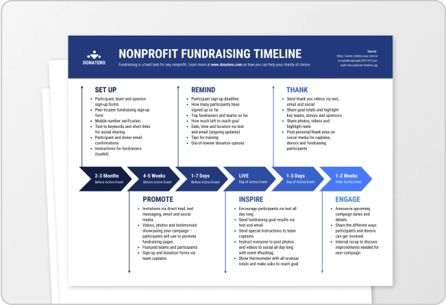
Timeline maker

Letterhead maker
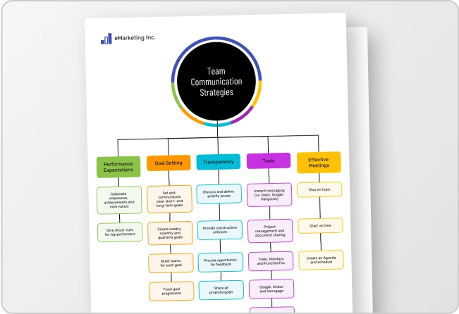
Mind map maker

Ebook maker
Data Topics
- Data Architecture
- Data Literacy
- Data Science
- Data Strategy
- Data Modeling
- Governance & Quality
- Education Resources For Use & Management of Data
Types of Data Visualization and Their Uses
In today’s data-first business environment, the ability to convey complex information in an understandable and visually appealing manner is paramount. Different types of data visualization help transform analyzed data into comprehensible visuals for all types of audiences, from novices to experts. In fact, research has shown that the human brain can process images in as little as […]

In today’s data-first business environment, the ability to convey complex information in an understandable and visually appealing manner is paramount. Different types of data visualization help transform analyzed data into comprehensible visuals for all types of audiences, from novices to experts. In fact, research has shown that the human brain can process images in as little as 13 milliseconds.

In essence, data visualization is indispensable for distilling complex information into digestible formats that support both quick comprehension and informed decision-making. Its role in analysis and reporting underscores its value as a critical tool in any data-centric activity.
Types of Data Visualization: Charts, Graphs, Infographics, and Dashboards
The diverse landscape of data visualization begins with simple charts and graphs but moves beyond infographics and animated dashboards. Charts , in their various forms – be it bar charts for comparing quantities across categories or line charts depicting trends over time – serve as efficient tools for data representation. Graphs extend this utility further: Scatter plots reveal correlations between variables, while pie graphs offer a visual slice of proportional relationships within a dataset.
Venturing beyond these traditional forms, infographics emerge as powerful storytelling tools, combining graphical elements with narrative to enlighten audiences on complex subjects. Unlike standard charts or graphs that focus on numerical data representation, infographics can incorporate timelines, flowcharts, and comparative images to weave a more comprehensive story around the data.
A dashboard, when effectively designed , serves as an instrument for synthesizing complex data into accessible and actionable insights. Dashboards very often encapsulate a wide array of information, from real-time data streams to historical trends, and present it through an amalgamation of charts, graphs, and indicators.
A dashboard’s efficacy lies in its ability to tailor the visual narrative to the specific needs and objectives of its audience. By selectively filtering and highlighting critical data points, dashboards facilitate a focused analysis that aligns with organizational goals or individual projects.
The best type of data visualization to use depends on the data at hand and the purpose of its presentation. Whether aiming to highlight trends, compare values, or elucidate complex relationships, selecting the appropriate visual form is crucial for effectively communicating insights buried within datasets. Through thoughtful design and strategic selection among these varied types of visualizations, one can illuminate patterns and narratives hidden within numbers – transforming raw data into meaningful knowledge.
Other Types of Data Visualization: Maps and Geospatial Visualization
Utilizing maps and geospatial visualization serves as a powerful method for uncovering and displaying insightful patterns hidden within complex datasets. At the intersection of geography and data analysis, this technique transforms numerical and categorical data into visual formats that are easily interpretable, such as heat maps, choropleths, or symbolic representations on geographical layouts. This approach enables viewers to quickly grasp spatial relationships, distributions, trends, and anomalies that might be overlooked in traditional tabular data presentations.
For instance, in public health, geospatial visualizations can highlight regions with high incidences of certain diseases, guiding targeted interventions. In environmental studies, they can illustrate changes in land use or the impact of climate change across different areas over time. By embedding data within its geographical context, these visualizations foster a deeper understanding of how location influences the phenomena being studied.
Furthermore, the advent of interactive web-based mapping tools has enhanced the accessibility and utility of geospatial visualizations. Users can now engage with the data more directly – zooming in on areas of interest, filtering layers to refine their focus, or even contributing their own data points – making these visualizations an indispensable tool for researchers and decision-makers alike who are looking to extract meaningful patterns from spatially oriented datasets.
Additionally, scatter plots excel in revealing correlations between two variables. By plotting data points on a two-dimensional graph, they allow analysts to discern potential relationships or trends that might not be evident from raw data alone. This makes scatter plots a staple in statistical analysis and scientific research where establishing cause-and-effect relationships is crucial.
Bubble charts take the concept of scatter plots further by introducing a third dimension – typically represented by the size of the bubbles – thereby enabling an even more layered understanding of data relationships. Whether it’s comparing economic indicators across countries or visualizing population demographics, bubble charts provide a dynamic means to encapsulate complex interrelations within datasets, making them an indispensable tool for advanced data visualization.
Innovative Data Visualization Techniques: Word Clouds and Network Diagrams
Some innovative techniques have emerged in the realm of data visualization that not only simplify complex datasets but also enhance engagement and understanding. Among these, word clouds and network diagrams stand out for their unique approaches to presenting information.
Word clouds represent textual data with size variations to emphasize the frequency or importance of words within a dataset. This technique transforms qualitative data into a visually appealing format, making it easier to identify dominant themes or sentiments in large text segments.
Network diagrams introduce an entirely different dimension by illustrating relationships between entities. Through nodes and connecting lines, they depict how individual components interact within a system – be it social networks, organizational structures, or technological infrastructures. This visualization method excels in uncovering patterns of connectivity and influence that might remain hidden in traditional charts or tables.
Purpose and Uses of Each Type of Data Visualization
The various types of data visualization – from bar graphs and line charts to heat maps and scatter plots – cater to different analytical needs and objectives. Each type is meticulously designed to highlight specific aspects of the data, making it imperative to understand their unique applications and strengths. This foundational knowledge empowers users to select the most effective visualization technique for their specific dataset and analysis goals.
Line Charts: Tracking Changes Over Time Line charts are quintessential in the realm of data visualization for their simplicity and effectiveness in showcasing trends and changes over time. By connecting individual data points with straight lines, they offer a clear depiction of how values rise and fall across a chronological axis. This makes line charts particularly useful for tracking the evolution of quantities – be it the fluctuating stock prices in financial markets, the ebb and flow of temperatures across seasons, or the gradual growth of a company’s revenue over successive quarters. The visual narrative that line charts provide helps analysts, researchers, and casual observers alike to discern patterns within the data, such as cycles or anomalies.
Bar Charts and Histograms: Comparing Categories and Distributions Bar charts are highly suitable for representing comparative data. By plotting each category of comparison with a bar whose height or length reflects its value, bar charts make it easy to visualize relative values at a glance.
Histograms show the distribution of groups of data in a dataset. This is particularly useful for understanding the shape of data distributions – whether they are skewed, normal, or have any outliers. Histograms provide insight into the underlying structure of data, revealing patterns that might not be apparent.
Pie Charts: Visualizing Proportional Data Pie charts serve as a compelling visualization tool for representing proportional data, offering a clear snapshot of how different parts contribute to a whole. By dividing a circle into slices whose sizes are proportional to their quantity, pie charts provide an immediate visual comparison among various categories. This makes them especially useful in illustrating market shares, budget allocations, or the distribution of population segments.
The simplicity of pie charts allows for quick interpretation, making it easier for viewers to grasp complex data at a glance. However, when dealing with numerous categories or when precise comparisons are necessary, the effectiveness of pie charts may diminish. Despite this limitation, their ability to succinctly convey the relative significance of parts within a whole ensures their enduring popularity in data visualization across diverse fields.
Scatter Plots: Identifying Relationship and Correlations Between Variables Scatter plots are primarily used for spotting relationships and correlations between variables. These plots show data points related to one variable on one axis and a different variable on another axis. This visual arrangement allows viewers to determine patterns or trends that might indicate a correlation or relationship between the variables in question.
For instance, if an increase in one variable consistently causes an increase (or decrease) in the other, this suggests a potential correlation. Scatter plots are particularly valuable for preliminary analyses where researchers seek to identify variables that warrant further investigation. Their straightforward yet powerful nature makes them indispensable for exploring complex datasets, providing clear insights into the dynamics between different factors at play.
Heat Maps: Representing Complex Data Matrices through Color Gradients Heat maps serve as a powerful tool in representing complex data matrices, using color gradients to convey information that might otherwise be challenging to digest. At their core, heat maps transform numerical values into a visual spectrum of colors, enabling viewers to quickly grasp patterns, outliers, and trends within the data. This method becomes more effective when the complex relationships between multiple variables need to be reviewed.
For instance, in fields like genomics or meteorology, heat maps can illustrate gene expression levels or temperature fluctuations across different regions and times. By assigning warmer colors to higher values and cooler colors to lower ones, heat maps facilitate an intuitive understanding of data distribution and concentration areas, making them indispensable for exploratory data analysis and decision-making processes.
Dashboards and Infographics: Integrating Multiple Data Visualizations Dashboards and infographics represent a synergistic approach in data visualization, blending various graphical elements to offer a holistic view of complex datasets. Dashboards, with their capacity to integrate multiple data visualizations such as charts, graphs, and maps onto a single interface, are instrumental in monitoring real-time data and tracking performance metrics across different parameters. They serve as an essential tool for decision-makers who require a comprehensive overview to identify trends and anomalies swiftly.
Infographics, on the other hand, transform intricate data sets into engaging, easily digestible visual stories. By illustrating strong narratives with striking visuals and solid statistics, infographics make complex information easily digestible to any type of audience.
Together, dashboards and infographics convey multifaceted data insights in an integrated manner – facilitating informed decisions through comprehensive yet clear snapshots of data landscapes.

Data visualization is the representation of data through use of common graphics, such as charts, plots, infographics and even animations. These visual displays of information communicate complex data relationships and data-driven insights in a way that is easy to understand.
Data visualization can be utilized for a variety of purposes, and it’s important to note that is not only reserved for use by data teams. Management also leverages it to convey organizational structure and hierarchy while data analysts and data scientists use it to discover and explain patterns and trends. Harvard Business Review (link resides outside ibm.com) categorizes data visualization into four key purposes: idea generation, idea illustration, visual discovery, and everyday dataviz. We’ll delve deeper into these below:
Idea generation
Data visualization is commonly used to spur idea generation across teams. They are frequently leveraged during brainstorming or Design Thinking sessions at the start of a project by supporting the collection of different perspectives and highlighting the common concerns of the collective. While these visualizations are usually unpolished and unrefined, they help set the foundation within the project to ensure that the team is aligned on the problem that they’re looking to address for key stakeholders.
Idea illustration
Data visualization for idea illustration assists in conveying an idea, such as a tactic or process. It is commonly used in learning settings, such as tutorials, certification courses, centers of excellence, but it can also be used to represent organization structures or processes, facilitating communication between the right individuals for specific tasks. Project managers frequently use Gantt charts and waterfall charts to illustrate workflows . Data modeling also uses abstraction to represent and better understand data flow within an enterprise’s information system, making it easier for developers, business analysts, data architects, and others to understand the relationships in a database or data warehouse.
Visual discovery
Visual discovery and every day data viz are more closely aligned with data teams. While visual discovery helps data analysts, data scientists, and other data professionals identify patterns and trends within a dataset, every day data viz supports the subsequent storytelling after a new insight has been found.
Data visualization
Data visualization is a critical step in the data science process, helping teams and individuals convey data more effectively to colleagues and decision makers. Teams that manage reporting systems typically leverage defined template views to monitor performance. However, data visualization isn’t limited to performance dashboards. For example, while text mining an analyst may use a word cloud to to capture key concepts, trends, and hidden relationships within this unstructured data. Alternatively, they may utilize a graph structure to illustrate relationships between entities in a knowledge graph. There are a number of ways to represent different types of data, and it’s important to remember that it is a skillset that should extend beyond your core analytics team.
Use this model selection framework to choose the most appropriate model while balancing your performance requirements with cost, risks and deployment needs.
Register for the ebook on generative AI
The earliest form of data visualization can be traced back the Egyptians in the pre-17th century, largely used to assist in navigation. As time progressed, people leveraged data visualizations for broader applications, such as in economic, social, health disciplines. Perhaps most notably, Edward Tufte published The Visual Display of Quantitative Information (link resides outside ibm.com), which illustrated that individuals could utilize data visualization to present data in a more effective manner. His book continues to stand the test of time, especially as companies turn to dashboards to report their performance metrics in real-time. Dashboards are effective data visualization tools for tracking and visualizing data from multiple data sources, providing visibility into the effects of specific behaviors by a team or an adjacent one on performance. Dashboards include common visualization techniques, such as:
- Tables: This consists of rows and columns used to compare variables. Tables can show a great deal of information in a structured way, but they can also overwhelm users that are simply looking for high-level trends.
- Pie charts and stacked bar charts: These graphs are divided into sections that represent parts of a whole. They provide a simple way to organize data and compare the size of each component to one other.
- Line charts and area charts: These visuals show change in one or more quantities by plotting a series of data points over time and are frequently used within predictive analytics. Line graphs utilize lines to demonstrate these changes while area charts connect data points with line segments, stacking variables on top of one another and using color to distinguish between variables.
- Histograms: This graph plots a distribution of numbers using a bar chart (with no spaces between the bars), representing the quantity of data that falls within a particular range. This visual makes it easy for an end user to identify outliers within a given dataset.
- Scatter plots: These visuals are beneficial in reveling the relationship between two variables, and they are commonly used within regression data analysis. However, these can sometimes be confused with bubble charts, which are used to visualize three variables via the x-axis, the y-axis, and the size of the bubble.
- Heat maps: These graphical representation displays are helpful in visualizing behavioral data by location. This can be a location on a map, or even a webpage.
- Tree maps, which display hierarchical data as a set of nested shapes, typically rectangles. Treemaps are great for comparing the proportions between categories via their area size.
Access to data visualization tools has never been easier. Open source libraries, such as D3.js, provide a way for analysts to present data in an interactive way, allowing them to engage a broader audience with new data. Some of the most popular open source visualization libraries include:
- D3.js: It is a front-end JavaScript library for producing dynamic, interactive data visualizations in web browsers. D3.js (link resides outside ibm.com) uses HTML, CSS, and SVG to create visual representations of data that can be viewed on any browser. It also provides features for interactions and animations.
- ECharts: A powerful charting and visualization library that offers an easy way to add intuitive, interactive, and highly customizable charts to products, research papers, presentations, etc. Echarts (link resides outside ibm.com) is based in JavaScript and ZRender, a lightweight canvas library.
- Vega: Vega (link resides outside ibm.com) defines itself as “visualization grammar,” providing support to customize visualizations across large datasets which are accessible from the web.
- deck.gl: It is part of Uber's open source visualization framework suite. deck.gl (link resides outside ibm.com) is a framework, which is used for exploratory data analysis on big data. It helps build high-performance GPU-powered visualization on the web.
With so many data visualization tools readily available, there has also been a rise in ineffective information visualization. Visual communication should be simple and deliberate to ensure that your data visualization helps your target audience arrive at your intended insight or conclusion. The following best practices can help ensure your data visualization is useful and clear:
Set the context: It’s important to provide general background information to ground the audience around why this particular data point is important. For example, if e-mail open rates were underperforming, we may want to illustrate how a company’s open rate compares to the overall industry, demonstrating that the company has a problem within this marketing channel. To drive an action, the audience needs to understand how current performance compares to something tangible, like a goal, benchmark, or other key performance indicators (KPIs).
Know your audience(s): Think about who your visualization is designed for and then make sure your data visualization fits their needs. What is that person trying to accomplish? What kind of questions do they care about? Does your visualization address their concerns? You’ll want the data that you provide to motivate people to act within their scope of their role. If you’re unsure if the visualization is clear, present it to one or two people within your target audience to get feedback, allowing you to make additional edits prior to a large presentation.
Choose an effective visual: Specific visuals are designed for specific types of datasets. For instance, scatter plots display the relationship between two variables well, while line graphs display time series data well. Ensure that the visual actually assists the audience in understanding your main takeaway. Misalignment of charts and data can result in the opposite, confusing your audience further versus providing clarity.
Keep it simple: Data visualization tools can make it easy to add all sorts of information to your visual. However, just because you can, it doesn’t mean that you should! In data visualization, you want to be very deliberate about the additional information that you add to focus user attention. For example, do you need data labels on every bar in your bar chart? Perhaps you only need one or two to help illustrate your point. Do you need a variety of colors to communicate your idea? Are you using colors that are accessible to a wide range of audiences (e.g. accounting for color blind audiences)? Design your data visualization for maximum impact by eliminating information that may distract your target audience.
An AI-infused integrated planning solution that helps you transcend the limits of manual planning.
Build, run and manage AI models. Prepare data and build models on any cloud using open source code or visual modeling. Predict and optimize your outcomes.
Unlock the value of enterprise data and build an insight-driven organization that delivers business advantage with IBM Consulting.
Your trusted Watson co-pilot for smarter analytics and confident decisions.
Use features within IBM Watson® Studio that help you visualize and gain insights into your data, then cleanse and transform your data to build high-quality predictive models.
Data Refinery makes it easy to explore, prepare, and deliver data that people across your organization can trust.
Learn how to use Apache Superset (a modern, enterprise-ready business intelligence web application) with Netezza database to uncover the story behind the data.
Predict outcomes with flexible AI-infused forecasting and analyze what-if scenarios in real-time. IBM Planning Analytics is an integrated business planning solution that turns raw data into actionable insights. Deploy as you need, on premises or on cloud.
What Is Data Visualization and Why Is It Important?
The sheer amount of data generated today means we need new ways to understand what’s happening in order to take action faster. Every click, transaction, subscription, loyalty card swipe, and social media interaction contributes to a digital footprint that continues to grow exponentially. The result? A massive explosion of data that is revolutionizing the way we live and work. Data visualization, in particular, plays a critical role in presenting data in a meaningful and understandable format. By using a visual representation of data , it’s much easier to identify patterns, trends, and relationships that may not be immediately apparent when sifting through large data sets.
Here’s what we’ll cover in this guide to data visualization:
- Data Visualization Definition
Benefits of Data Visualization
Why data visualization is important .
- Types of Data Visualization and Examples
- Evaluating Data Visualization Tools
- Take the Next Step and Start Analyzing With Data Visualization
Data Visualization Definition
Data visualization is the process of transforming raw data into visual formats, such as charts, graphs, or maps, to help identify patterns, trends, and insights that might not be apparent from numerical data alone.
Additionally, it enables data to be more accessible, understandable, and impactful, especially when communicating with stakeholders, investors, or team members who may not be familiar with the data.
For example, data visualization could help:
- In retail, gaining insights into customer behavior, purchase patterns, and product performance.
- In finance, monitoring market trends, tracking portfolio performance, and conducting risk analysis.
- In public health, showing the geographical distribution of outbreaks and helping track the spread of infectious diseases.
- In supply chain industries, tracking inventory levels, monitoring logistics operations, and optimizing resource allocation.
- In sports, evaluating player performance, game strategies, and match statistics.
- In education, tracking student performance, analyzing learning outcomes, and identifying areas for improvement.
Data visualization has several benefits for businesses including: the ability to process information faster, identify trends at scale, and make data more digestible. Companies regularly use data to make decisions, and through data visualization, can find insights quickly and move to action. Data visualization specifically helps with the following:
- Visualizing patterns and relationships
- Storytelling, including specifically data storytelling
- Accessibility to information
Exploration
Let’s take a look at each of these benefits in detail.
Visualize patterns and relationships
Data visualization constitutes an excellent method for the discernment of interconnections and patterns amidst vast collections of information. For example, a scatter plot can be used to display the relationship between two variables, such as the correlation between temperature and sales. This enables users to understand the relationship and identify trends and outliers more quickly and easily.
Read a guide of Sigma’s visual library.

Storytelling
Your audience, whether it's coworkers or clients, want to hear a coherent story from your data. Storytelling with data cannot be done successfully without visualizations. Colorful charting and dynamic pivots are just as important as characters and plots are in a traditional story, so using them to communicate information makes data that much more engaging and memorable for audiences. Data can be complex and convoluted for some audiences, so data storytelling is an approach to convey important information effectively through a captivating narrative. Good visualizations are a vital part of that narrative.
For example, if an analyst is investigating the performance of e-commerce sales for their retail company over time, they may leverage several data sources such as spreadsheets, calculations, code, etc. to do so. However, when they report these new insights to their stakeholders, the analyst will need to summarize and communicate their findings in a digestible way.
An easy way the analyst could do this is by using the data to create a map of the U.S. with a color gradient overlaying every state that is lighter or darker based on its total sales volume. This visual story tells the least and most successful retail locations at a glance.

Accessibility / Easily Share Information
Data visualization serves as an invaluable mechanism for the facilitation of accessibility, allowing for the communication of information amongst individuals, even for those who may not usually engage with data , which broadens the audience.
Visualizations help simplify complex information by leveraging people’s ability to naturally recognize patterns. A viewer typically does not have to be taught that bigger means more and that smaller means less. In a case where an analyst wants to highlight the difference in scale between one product’s profitability vs. another, a bar chart can clearly show the user which product is more profitable and by how much, making it easy for even non-technical team members to understand and compare the performance of different products.
Exploration is a key component of successful data visualization. The more flexible charting and dashboarding is, the more follow-up questions end users can ask directly of their data. For example, an interactive dashboard can be used to explore retail sales data over time, enabling users to filter and drill down into the data to identify trends and patterns.
Data visualization exploration is often associated with the concept of “drill downs.” Drill downs in data visualization refer to the process of starting with an overview of data and then narrowing the focus to more specific aspects of it. As an example, one might start with a visualization of global climate data and drill down to data about a specific country, a specific state, a specific city, or even a specific neighborhood within that city. Each drill down reveals more precise, detailed, and nuanced information.
The main goal of data visualization is that it helps unify and bring teams onto the same page. The human mind is wired to grasp visual information more effortlessly than raw data in spreadsheets or detailed reports. Thus, graphical representation of voluminous and intricate data is more user-friendly. Data visualization offers a swift and straightforward method to communicate ideas in a universally understood format, with the added benefit of enabling scenario testing through minor modifications.
By translating information into visual form, it ensures everyone, irrespective of the complexity of the data or the depth of the analysis, can share a unified understanding. Any industry can benefit from using data visualization, because pretty much every industry relies on data to power it. That includes finance, marketing, consumer goods, education, government, sports, history, and many more. Another thing to keep in mind is that data visualization can be a double-edged sword. For example, charts can be manipulated and skewed to force a desired outcome. Ungoverned, static, desktop tools can become the wild west in suggesting an inaccurate outcome “proven by data.” Even in the cases where the visualization builder is acting in good faith, there are still pitfalls to watch out for. Always be considerate of:
- Individual outliers having an outsized impact, skewing the visual direction of a chart
- The need for for business users to see the underlying data
- Allowing for transparency down to row-level detail in data sets

Types of Data Visualizations & Examples
There is a long list of types of data visualization techniques and methods that can be used to represent data. While no type of data visualization is perfect, we’ll walk through different examples and when to apply each one.
We’ll be looking at:
- Line charts and area charts
- Scatter plots
- Pivot tables
- Box-and-whisker plots
- Sankey charts
Tables, although more commonly thought of as a data source, can also be considered a type of data visualization. Especially when conditional formatting is applied to the table’s rows and columns, the data within the table becomes more visually engaging and informative. With conditional formatting, important insights and patterns can be highlighted, making it easier for viewers to identify trends and outliers at a glance. Additionally, tables offer a structured and organized way to present information, allowing for a comprehensive comparison of data points, which further enhances data understanding and analysis. For example, Sigma’s UI is based on a spreadsheet-like interface, which means almost everything in Sigma begins in a table format. That said, you can also create visual tables that display a smaller amount of data in order to tell a clearer story. In data visualization, tables are a simplified way of representing this interface.
When to use tables:
- For detailed numeric comparisons, or when precision of data is key
- For displaying multidimensional data; tables can handle this complexity quite well
When to avoid tables:
- When patterns, trends, or relationships need to be highlighted at a glance
- When dealing with large amounts of data

Pie charts —similar to stacked bar charts—are useful for displaying categorical data, such as market share or customer demographics. Pie charts are often used to display data that can be divided into categories or subgroups, and to show how each category or subgroup contributes to the whole. For example, a pie chart could be used to show the proportion of sales for different product categories in a given period of time, or the percent of a company's revenue broken down by various regions.
When to use pie charts:
- You want to display a proportion or percentage of a whole
- You’re visualizing only seven categories or less
When to avoid pie charts:
- You’re visualizing more than seven categories
- You want to compare something with more details, rather than just proportion
- You want to display and pinpoint exact values

A bar chart, or bar graph, constitutes a variety of graphs that employ rectangular bars to depict data. These bars can be oriented either horizontally or vertically, with their extent being directly proportional to the numerical values they are intended to embody. Predominantly utilized for juxtaposing data across disparate categories or illustrating shifts in data over temporal progressions, bar charts offer a straightforward, yet potent means of conveying information visually. They frequently function as the initial tool in the exploratory process of data investigation.
When to use bar charts:
- Emphasizing and contrasting different sets of data, making the disparities or similarities between categories clear
- To display a subset of a larger dataset
When to avoid bar charts:
- When a particular field encompasses an overwhelming variety of data types
- When the differences between fields are too subtle, or when these differences exist on different scales, as it could lead to confusion or misinterpretation
Line Charts & Area Charts

Line charts and area charts are two types of charts that are commonly used to visualize data trends over time. A line chart, also called a line graph, is a distinct type of graphical representation that exhibits information in the form of a multitude of data points, which are interconnected by unbroken lines. These line charts are typically employed to demonstrate transformations in data over a certain duration, where the horizontal axis symbolizes time, and the vertical axis signifies the values under scrutiny. Furthermore, they can serve to juxtapose several series of data within the same chart, or to graphically illustrate predicted time periods.
For example, a line chart can be used to visualize a company's stock prices over the course of a year. Similarly, an area chart can be used to visualize the temperature changes over a day.
When to use line charts:
- When you’re displaying time-based continuous data
- When you have multiple series or larger datasets
When to avoid line charts:
- When you have smaller datasets, bar charts are likely a better way to present the information
- Avoid when you need to compare multiple categories at once

When to use area charts:
- When you want to display the volume of the data you have
- When comparing data across more than one time period
When to avoid area charts:
- Avoid if you need to compare multiple categories, as well as when you need to examine the specific data value
Scatter Plots

A scatter plot , also called a scatter chart or scatter graph, is a specialized form of chart that demonstrates the correlation between two distinct variables by mapping them as a succession of individual data points. Each data point denotes a combined value of the two variables, with its specific placement within the chart dictated by these values.
Scatter charts prove instrumental in discerning patterns and trends within data, and they also help us understand how strong and in what direction the relationship is between two variables. They also serve as effective tools for identifying outliers, or those data points that deviate significantly from anticipated values based on the pattern displayed by other data points. These charts find widespread use across a range of fields including, but not limited to, statistics, engineering, and social sciences, for the purpose of analyzing and visualizing intricate data sets. In the realm of business, they are frequently utilized to identify correlations between different variables, for instance, examining the relationship between marketing outlays and resultant sales revenue. For example, a scatter plot might be used to visualize the relationship between the age and income of a group of people. Another example would be to plot the correlation between the amount of rainfall and the crop yield for a particular region.
When to use scatter plots:
- Highlight correlations within your data
- They are useful tools for statistical investigations
- Consider scatter plots to reveal underlying patterns or trends
When to avoid scatter plots:
- For smaller datasets, scatter plots may not be optimal
- Avoid scatter plots for excessively large datasets to prevent unintelligible data clustering
- If your data lacks correlations, scatter plots may not be the best choice
Pivot Tables
While pivot tables may not be what first comes to mind for data visualization, they can give important context with hard numbers and provide strong visual indicators through formatting. Pivot tables can also be enhanced with conditional formatting to provide color scales that make performance trends more visible. Data bars can also be added to cells to run either red or green for positive and negative values.
When to Use Pivot Tables:
- Cohort analysis performance trends or portfolio analysis with a mix of positive and negative values
What Not to Use Pivot Tables:
- When your dataset is too large to get a good understanding of the whole
- When data can easily be summarized with a bar chart instead

An example of a pivot table, where colors are used to show positive or negative progress on a company’s portfolio. The user can pivot the table to show multiple categories in different ways.
A heat map is a type of chart that uses color to represent data values. It is often used to visualize data that is organized in a matrix or table format. The color of each cell in the matrix is determined by the value of the corresponding data point. Heat maps are best used when analyzing data that is organized in a two-dimensional grid or matrix.
For example, a heat map can be used to visualize a company's website traffic, where the rows represent different pages on the website, and the columns represent different periods of time.
When to use heat maps:
- When you need to visualize the density or intensity of variables
- When you want to display patterns or trends over time or space
When to avoid heat maps:
- When precise values are needed; heat maps are better at showing relative differences rather than precise values
- When working with small data sets
A tree map is a type of chart that is used to visualize hierarchical data. It consists of a series of nested rectangles, where the size and color of each rectangle represent a different variable. Tree maps are best used when analyzing data that has a hierarchical structure.
For example, a tree map can be used to visualize the market share of different companies in an industry. The largest rectangle would represent the entire industry, with smaller rectangles representing the market share of each individual company.
When to use tree maps:
- When you want to visualize hierarchical data
- When you need to illustrate the proportion of different categories within a whole
When to avoid tree maps:
- When exact values are important
- When there are too many categories
Box-and-Whisker Plots

Box plots are useful for quickly summarizing the distribution of a dataset, particularly its central tendency and variability. For example, a box-and-whisker plot can be used to visualize the test scores of a group of students.
Colloquially recognized as a box-and-whisker plot, a box plot is a distinct form of chart that showcases the distribution of a collection of numerical data through its quartile divisions. Box plots serve as efficient tools for rapidly encapsulating the distribution of a dataset, specifically its central propensity and variability.
A box-and-whisker plot consists of a rectangle (the "box") and a pair of "whiskers" that extend from it. The box embodies the middle 50% of the data, with the lower boundary of the box signaling the first quartile (25th percentile) and the upper boundary of the box indicating the third quartile (75th percentile). The line situated within the box signifies the median value of the data. The whiskers project from the box to the minimum and maximum values of the data, or to a designated distance from the box referred to as the "fences." Any data points that reside outside the whiskers or fences are categorized as outliers and are plotted as individual points. When to use box plot charts:
- When you want to display data spread and skewness
- When showcasing the distribution of data, including the range, quartiles, and potential outliers
- When comparing multiple groups or categories side-by-side; they allow for easy comparison of different distributions.
When to avoid box plot charts:
- If you need to show more detail, since box plots focus on a high-level summary
- When individual data points are important to the story you’re telling
- When your audience isn’t familiar with them, since they can sometimes be less intuitive than other types of visualizations
A histogram is a type of chart that displays the distribution of a dataset. It consists of a series of vertical bars, where the height of each bar represents the number of observations in a particular range. Histograms are best used when analyzing continuous data. It’s used the most when you want to understand the frequency distribution of a numerical variable, like height, weight, or age. For example, a histogram can be used to visualize the distribution of heights in a population. Read more about building histograms in Sigma here.
When to Use a Histogram:
- When understanding the shape of a distribution; for example, whether it’s symmetric, skewed to the left or right, or bimodal
- When identifying outliers, like which data points are significantly different from the rest of the data
- When comparing distribution of a variable across different groups, such as males and females, or different age groups.
- To set boundaries for data ranges; for example, you might use a histogram to determine what constitutes a "normal" or "abnormal" value for a particular variable
When to Avoid a Histogram:
- When you need to look at multiple dimensions at the same time
- If your data isn’t all on the same scale
Sankey Charts

We end our guide with the controversial Sankey chart. A Sankey chart is a type of diagram that illustrates the movement or transfer of data, resources, or quantities through various stages of a system or process. Common applications of Sankey charts include visualizing complex sequences like energy usage, material distribution, or even a website's user journey. The structure of the chart includes nodes and links—with nodes representing the starting points, endpoints, or intermediate steps, and links depicting the transition of quantities or data between these nodes.
The thickness of the links in a Sankey chart directly corresponds to the volume of data or resources being moved, offering an intuitive comparison of the relative sizes of these transfers. They can be invaluable for recognizing inefficiencies, bottlenecks, or potential areas for enhancement in a system or process. These charts serve as a powerful tool for communicating complex information in a straightforward and comprehensible way. However, if there are too many nodes or links, Sankey charts can become cluttered and challenging to interpret, hence their use should be considerate and targeted.
When to use Sankey charts:
- When you want to show the data as part of a process
When to avoid Sankey charts:
- When it starts to feel too confusing, which can quickly happen when there are too many nodes or links
- When you need to see exact values, it might not be the most intuitive option.
Evaluating Data Visualization Tools
Data visualization tools have become increasingly popular in recent years, with a wide variety of options available to choose from. However, determining which tool best suits your needs can be challenging with so many options. When evaluating data visualization tools, there are several key questions to consider:
- What are your goals and needs? It's crucial to clearly understand your goals and needs before selecting a data visualization tool. Are you looking to explore your data, communicate a specific message, or both? Understanding your objectives will help you choose the right tool for your project.
- What features do you require? Different data visualization tools come with different features. Before selecting a tool, you should consider what features you need to achieve your goals. For example, do you require interactive capabilities or the ability to create custom visualizations?
- Where will your data come from? The source of your data is another critical factor to consider when selecting a data visualization tool. Some tools are better suited for specific types of data, such as structured or unstructured data, while others may require specific file formats or data storage solutions.
- Where will you need to see your data? Different data visualization tools may be more suitable for specific platforms or devices. For example, some tools may be optimized for mobile devices, while others are designed for desktop computers or specific web browsers. You may also be interested in embedding visualizations elsewhere , such as internal applications or external portals.
- Where would you like to publish your visualization? Finally, consider where you would like to publish your visualization. Some tools may provide built-in publishing capabilities, while others may require you to export your visualization to a separate platform. Selecting a tool that supports your publishing needs is important to ensure your visualization reaches your intended audience.
By considering these key questions, you can evaluate different data visualization tools and select the one that best meets your needs.
Read a side-by-side comparison of Sigma against similar BI tools.
Take the Next Step & Start Analyzing With Data Visualization
Data visualization is a powerful tool for understanding and communicating complex data. While there are many data visualization tools on the market, Sigma offers an intuitive and familiar spreadsheet interface that allows users to easily explore, analyze, and collaborate on their data.
Explore Sigma’s capabilities and start transforming your data today via a free trial of Sigma .
Related resources
.webp)
This is the default text value
Watch on-DEMAND DEMOS
ATTEND AN EVENT
Get a free trial
INTERACTIVE DEMOS
JOIN THE COMMUNITY
SCHEDULE A CALL
ATTEND A LIVE LAB
SEE WORKBOOK EXAMPLES
JOIN THE SIGMA COMMUNITY
- X (Twitter)
Painting Pictures with Data: The Power of Visual Representations

Picture this. A chaotic world of abstract concepts and complex data, like a thousand-piece jigsaw puzzle. Each piece, a different variable, a unique detail.
Alone, they’re baffling, nearly indecipherable.
But together? They’re a masterpiece of visual information, a detailed illustration.
American data pioneer Edward Tufte , a notable figure in the graphics press, believed that the art of seeing is not limited to the physical objects around us. He stated, “The commonality between science and art is in trying to see profoundly – to develop strategies of seeing and showing.”
It’s in this context that we delve into the world of data visualization. This is a process where you create visual representations that foster understanding and enhance decision making.
It’s the transformation of data into visual formats. The information could be anything from theoretical frameworks and research findings to word problems. Or anything in-between. And it has the power to change the way you learn, work, and more.
And with the help of modern technology, you can take advantage of data visualization easier than ever today.
What are Visual Representations?
Think of visuals, a smorgasbord of graphical representation, images, pictures, and drawings. Now blend these with ideas, abstract concepts, and data.
You get visual representations . A powerful, potent blend of communication and learning.
As a more formal definition, visual representation is the use of images to represent different types of data and ideas.
They’re more than simply a picture. Visual representations organize information visually , creating a deeper understanding and fostering conceptual understanding. These can be concrete objects or abstract symbols or forms, each telling a unique story. And they can be used to improve understanding everywhere, from a job site to an online article. University professors can even use them to improve their teaching.
But this only scratches the surface of what can be created via visual representation.
Types of Visual Representation for Improving Conceptual Understanding
Graphs, spider diagrams, cluster diagrams – the list is endless!
Each type of visual representation has its specific uses. A mind map template can help you create a detailed illustration of your thought process. It illustrates your ideas or data in an engaging way and reveals how they connect.
Here are a handful of different types of data visualization tools that you can begin using right now.
1. Spider Diagrams

Spider diagrams , or mind maps, are the master web-weavers of visual representation.
They originate from a central concept and extend outwards like a spider’s web. Different ideas or concepts branch out from the center area, providing a holistic view of the topic.
This form of representation is brilliant for showcasing relationships between concepts, fostering a deeper understanding of the subject at hand.
2. Cluster Diagrams

As champions of grouping and classifying information, cluster diagrams are your go-to tools for usability testing or decision making. They help you group similar ideas together, making it easier to digest and understand information.
They’re great for exploring product features, brainstorming solutions, or sorting out ideas.
3. Pie Charts

Pie charts are the quintessential representatives of quantitative information.
They are a type of visual diagrams that transform complex data and word problems into simple symbols. Each slice of the pie is a story, a visual display of the part-to-whole relationship.
Whether you’re presenting survey results, market share data, or budget allocation, a pie chart offers a straightforward, easily digestible visual representation.
4. Bar Charts

If you’re dealing with comparative data or need a visual for data analysis, bar charts or graphs come to the rescue.
Bar graphs represent different variables or categories against a quantity, making them perfect for representing quantitative information. The vertical or horizontal bars bring the data to life, translating numbers into visual elements that provide context and insights at a glance.
Visual Representations Benefits
1. deeper understanding via visual perception.
Visual representations aren’t just a feast for the eyes; they’re food for thought. They offer a quick way to dig down into more detail when examining an issue.
They mold abstract concepts into concrete objects, breathing life into the raw, quantitative information. As you glimpse into the world of data through these visualization techniques , your perception deepens.
You no longer just see the data; you comprehend it, you understand its story. Complex data sheds its mystifying cloak, revealing itself in a visual format that your mind grasps instantly. It’s like going from a two dimensional to a three dimensional picture of the world.
2. Enhanced Decision Making
Navigating through different variables and relationships can feel like walking through a labyrinth. But visualize these with a spider diagram or cluster diagram, and the path becomes clear. Visual representation is one of the most efficient decision making techniques .
Visual representations illuminate the links and connections, presenting a fuller picture. It’s like having a compass in your decision-making journey, guiding you toward the correct answer.
3. Professional Development
Whether you’re presenting research findings, sharing theoretical frameworks, or revealing historical examples, visual representations are your ace. They equip you with a new language, empowering you to convey your message compellingly.
From the conference room to the university lecture hall, they enhance your communication and teaching skills, propelling your professional development. Try to create a research mind map and compare it to a plain text document full of research documentation and see the difference.
4. Bridging the Gap in Data Analysis
What is data visualization if not the mediator between data analysis and understanding? It’s more than an actual process; it’s a bridge.
It takes you from the shores of raw, complex data to the lands of comprehension and insights. With visualization techniques, such as the use of simple symbols or detailed illustrations, you can navigate through this bridge effortlessly.
5. Enriching Learning Environments
Imagine a teaching setting where concepts are not just told but shown. Where students don’t just listen to word problems but see them represented in charts and graphs. This is what visual representations bring to learning environments.
They transform traditional methods into interactive learning experiences, enabling students to grasp complex ideas and understand relationships more clearly. The result? An enriched learning experience that fosters conceptual understanding.
6. Making Abstract Concepts Understandable
In a world brimming with abstract concepts, visual representations are our saving grace. They serve as translators, decoding these concepts into a language we can understand.
Let’s say you’re trying to grasp a theoretical framework. Reading about it might leave you puzzled. But see it laid out in a spider diagram or a concept map, and the fog lifts. With its different variables clearly represented, the concept becomes tangible.
Visual representations simplify the complex, convert the abstract into concrete, making the inscrutable suddenly crystal clear. It’s the power of transforming word problems into visual displays, a method that doesn’t just provide the correct answer. It also offers a deeper understanding.
How to Make a Cluster Diagram?
Ready to get creative? Let’s make a cluster diagram.
First, choose your central idea or problem. This goes in the center area of your diagram. Next, think about related topics or subtopics. Draw lines from the central idea to these topics. Each line represents a relationship.

While you can create a picture like this by drawing, there’s a better way.
Mindomo is a mind mapping tool that will enable you to create visuals that represent data quickly and easily. It provides a wide range of templates to kick-start your diagramming process. And since it’s an online site, you can access it from anywhere.
With a mind map template, creating a cluster diagram becomes an effortless process. This is especially the case since you can edit its style, colors, and more to your heart’s content. And when you’re done, sharing is as simple as clicking a button.
A Few Final Words About Information Visualization
To wrap it up, visual representations are not just about presenting data or information. They are about creating a shared understanding, facilitating learning, and promoting effective communication. Whether it’s about defining a complex process or representing an abstract concept, visual representations have it all covered. And with tools like Mindomo , creating these visuals is as easy as pie.
In the end, visual representation isn’t just about viewing data, it’s about seeing, understanding, and interacting with it. It’s about immersing yourself in the world of abstract concepts, transforming them into tangible visual elements. It’s about seeing relationships between ideas in full color. It’s a whole new language that opens doors to a world of possibilities.
The correct answer to ‘what is data visualization?’ is simple. It’s the future of learning, teaching, and decision-making.
Keep it smart, simple, and creative! The Mindomo Team
Related Posts

Top 5 Fishbone Diagram Templates You Need To Know About!

Mastering Your Mind: Exploring Effective Visualization Techniques

The Power of an Idea Map: Your Guide to Creative Thinking & Organizing Ideas

Innovation Unleashed: Mind Mapping vs Brainstorming in the Generation of Game-Changing Ideas

The Key to Success with Ingredients for a Fulfilling Life

Cracking the Code to Creative Thinking: Ignite Your Brain and Unleash Your Ideas
Write a comment cancel reply.
Save my name, email, and website in this browser for the next time I comment.
- Data Science
- Data Analysis
- Data Visualization
- Machine Learning
- Deep Learning
- Computer Vision
- Artificial Intelligence
- AI ML DS Interview Series
- AI ML DS Projects series
- Data Engineering
- Web Scrapping
Charts and Graphs for Data Visualization
As companies and groups deal with more and more data, it’s crucial to present it visually. Data is everywhere these days, and it can be overwhelming.
This article is your guide to Data Visualization , which is turning all that data into pictures and charts that are easy to understand. Whether you work in business, marketing, or anything else, these charts can help you explain ideas, track how things are going, and make smart choices.
What is Data Visualization?
Data visualization is taking a bunch of numbers and information and turning it into pictures or any kind of charts that are easier to understand. It takes a big pile of information and sorts it into pictures (like bar charts, line graphs, or pie charts) that make it easier to understand or see patterns and trends. Here are some of the things data visualization can help you see:
- How things are changing over time
- How things compare to each other
- Relationships between things
Different Types of Graphs for Data Visualization
Data can be a jumble of numbers and facts. Charts and graphs turn that jumble into pictures that make sense. 10 prime super useful chart types are:
Bar graphs are one of the most commonly used types of graphs for data visualization. They represent data using rectangular bars where the length of each bar corresponds to the value it represents. Bar graphs are effective for comparing data across different categories or groups.

Bar Graph Example
Advantages of Bar Graphs
- Highlighting Trends : Bar graphs are effective at highlighting trends and patterns in data, making it easy for viewers to identify relationships and comparisons between different categories or groups.
- Customizations : Bar graphs can be easily customized to suit specific visualization needs, such as adjusting colors, labels, and styles to enhance clarity and aesthetics.
- Space Efficiency : Bar graphs can efficiently represent large datasets in a compact space, allowing for the visualization of multiple variables or categories without overwhelming the viewer.
Disadvantages of Bar Graphs
- Limited Details : Bar graphs may not provide detailed information about individual data points within each category, limiting the depth of analysis compared to other visualization methods.
- Misleading Scaling : If the scale of the y-axis is manipulated or misrepresented, bar graphs can potentially distort the perception of data and lead to misinterpretation.
- Overcrowding : When too many categories or variables are included in a single bar graph, it can become overcrowded and difficult to read, reducing its effectiveness in conveying clear insights.
Line Graphs
Line graphs are used to display data over time or continuous intervals. They consist of points connected by lines, with each point representing a specific value at a particular time or interval. Line graphs are useful for showing trends and patterns in data. Perfect for showing trends over time, like tracking website traffic or how something changes.

Line Graph Example
Advantages of Line Graphs
- Clarity : Line graphs provide a clear representation of trends and patterns over time or across continuous intervals.
- Visual Appeal : The simplicity and elegance of line graphs make them visually appealing and easy to interpret.
- Comparison : Line graphs allow for easy comparison of multiple data series on the same graph, enabling quick insights into relationships and trends.
Disadvantages of Line Graphs
- Data Simplification: Line graphs may oversimplify complex data sets, potentially obscuring nuances or outliers.
- Limited Representation : Line graphs are most effective for representing continuous data over time or intervals and may not be suitable for all types of data, such as categorical or discrete data.
Different Types of Charts for Data Visualization
Pie charts are circular graphs divided into sectors, where each sector represents a proportion of the whole. The size of each sector corresponds to the percentage or proportion of the total data it represents. Pie charts are effective for showing the composition of a whole and comparing different categories as parts of a whole.

Pie Chart Example
Advantages of Pie Charts
- Easy to create: Pie charts can be quickly generated using various software tools or even by hand, making them accessible for visualizing data without specialized knowledge or skills.
- Visually appealing: The circular shape and vibrant colors of pie charts make them visually appealing, attracting the viewer’s attention and making the data more engaging.
- Simple and easy to understand: Pie charts present data in a straightforward manner, making it easy for viewers to grasp the relative proportions of different categories at a glance.
Disadvantages of Using a Pie Chart
- Limited trend analysis: Pie charts are not ideal for showing trends or changes over time since they represent static snapshots of data at a single point in time.
- Limited data slice: Pie charts become less effective when too many categories are included, as smaller slices can be difficult to distinguish and interpret accurately. They are best suited for representing a few categories with distinct differences in proportions.
Scatter Plots
Scatter plots are used to visualize the relationship between two variables. Each data point in a scatter plot represents a value for both variables, and the position of the point on the graph indicates the values of the variables. Scatter plots are useful for identifying patterns and relationships between variables, such as correlation or trends.

Scatter Chart Example
Advantages of Using Scatter Plots
- Revealing Trends and Relationships: Scatter plots are excellent for visually identifying patterns, trends, and relationships between two variables. They allow for the exploration of correlations and dependencies within the data.
- Easy to Understand: Scatter plots provide a straightforward visual representation of data points, making them easy for viewers to interpret and understand without requiring complex statistical knowledge.
- Highlight Outliers: Scatter plots make it easy to identify outliers or anomalous data points that deviate significantly from the overall pattern. This can be crucial for detecting unusual behavior or data errors within the dataset.
Disadvantages of Using Scatter Plot Charts
- Limited to Two Variables: Scatter plots are limited to visualizing relationships between two variables. While this simplicity can be advantageous for focused analysis, it also means they cannot represent interactions between more than two variables simultaneously.
- Not Ideal for Precise Comparisons: While scatter plots are excellent for identifying trends and relationships, they may not be ideal for making precise comparisons between data points. Other types of graphs, such as bar charts or box plots, may be better suited for comparing specific values or distributions within the data.
Area Charts
Area charts are similar to line graphs but with the area below the line filled in with color. They are used to represent cumulative totals or stacked data over time. Area charts are effective for showing changes in composition over time and comparing the contributions of different categories to the total.

Area Chart Example
Advantages of Using Area Charts
- Visually Appealing: Area charts are aesthetically pleasing and can effectively capture the audience’s attention due to their colorful and filled-in nature.
- Great for Trends: They are excellent for visualizing trends over time, as the filled area under the line emphasizes the magnitude of change, making it easy to identify patterns and fluctuations.
- Compares Well: Area charts allow for easy comparison between different categories or datasets, especially when multiple areas are displayed on the same chart. This comparative aspect aids in highlighting relative changes and proportions.
Disadvantages of Using Area Charts
- Limited Data Sets: Area charts may not be suitable for displaying large or complex datasets, as the filled areas can overlap and obscure details, making it challenging to interpret the data accurately.
- Not for Precise Values: Area charts are less effective for conveying precise numerical values, as the emphasis is on trends and proportions rather than exact measurements. This can be a limitation when precise data accuracy is crucial for analysis or decision-making.
Radar Charts
A radar chart , also known as a spider chart or a web chart, is a graphical method of displaying multivariate data in the form of a two-dimensional chart. It is particularly useful for visualizing the relative values of multiple quantitative variables across several categories. Radar charts compare things across many aspects, like how different employees perform in various skills.

Radar Chart Example
Advantages of Using Radar Chart
- Highlighting Strengths and Weaknesses: Radar charts allow for the clear visualization of strengths and weaknesses across multiple variables, making it easy to identify areas of excellence and areas for improvement.
- Easy Comparisons: The radial nature of radar charts facilitates easy comparison of different variables or categories, as each axis represents a different dimension of the data, enabling quick visual assessment.
- Handling Many Variables: Radar charts are particularly useful for handling datasets with many variables, as each variable can be represented by a separate axis, allowing for comprehensive visualization of multidimensional data.
Disadvantages of Using Radar Chart
- Scaling Issues: Radar charts can present scaling issues, especially when variables have different units or scales. Inaccurate scaling can distort the representation of data, leading to misinterpretation or misunderstanding.
- Misleading Comparisons: Due to the circular nature of radar charts, the area enclosed by each shape can be misleading when comparing variables. Small differences in values can result in disproportionately large visual differences, potentially leading to misinterpretation of data.
Histograms are similar to bar graphs but are used specifically to represent the distribution of continuous data. In histograms, the data is divided into intervals, or bins, and the height of each bar represents the frequency or count of data points within that interval.

Example of Histogram
Advantages of using Histogram
- Easy to understand: Histograms provide a visual representation of the distribution of data, making it easy for viewers to grasp the overall pattern.
- Identify Patterns: Histograms allow for the identification of patterns and trends within the data, such as skewness, peaks, or gaps.
- Compare Data Sets: Histograms enable comparisons between different datasets, helping to identify similarities or differences in their distributions.
Disadvantages of using Histogram
- Not for small datasets: Histograms may not be suitable for very small datasets as they require a sufficient amount of data to accurately represent the distribution.
- Limited details: Histograms provide a summary of the data distribution but may lack detailed information about individual data points, such as specific values or outliers.
Treemap Charts
Treemap charts are a type of data visualization that represent hierarchical data as a set of nested rectangles. Each rectangle, or “tile,” in the treemap represents a category or subcategory of the data, and the size of the rectangle corresponds to a quantitative value, such as the proportion or absolute value of that category within the dataset.

Treemap Charts >>
Advantages of using a Treemap Chart
- Identifying patterns and trends: Treemap charts help in visually identifying patterns and trends within hierarchical data structures by representing data in nested rectangles, making it easier to see how smaller components contribute to the whole.
- Highlighting Proportions: Treemaps effectively highlight proportions by using varying sizes and colors of rectangles to represent different values or categories, making it easy to understand the relative significance of each component.
- Efficient use of space: Treemap charts efficiently utilize space by packing rectangles within larger rectangles, allowing for the visualization of large datasets in a compact and organized manner.
Disadvantages of using a Treemap Chart
- Difficulty comparing exact values: Due to the varying sizes and shapes of the rectangles in a treemap, it can be challenging to accurately compare exact values between different categories or components, especially when the differences are subtle.
- Order dependence: The arrangement of rectangles within a treemap can significantly impact perception. Small changes in sorting or hierarchical structure can lead to different visual interpretations, making it important to carefully consider the ordering of data elements.
Pareto Charts
A Pareto chart is a specific type of chart that combines both bar and line graphs. It’s named after Vilfredo Pareto, an Italian economist who first noted the 80/20 principle, which states that roughly 80% of effects come from 20% of causes. Pareto charts are used to highlight the most significant factors among a set of many factors.

Pareto Chart Example
Advantages of using a Pareto Chart
- Simple to understand: Pareto charts present data in a straightforward manner, making it easy for viewers to grasp the most significant factors at a glance.
- Visually identify key factors: By arranging data in descending order of importance, Pareto charts allow users to quickly identify the most critical factors contributing to a problem or outcome.
- Focus resources effectively: With the ability to prioritize factors based on their impact, Pareto charts help organizations allocate resources efficiently by addressing the most significant issues first.
Disadvantages of Using a Pareto Chart
- Limited Data Exploration: Pareto charts primarily focus on identifying the most critical factors, which may lead to overlooking nuances or subtle trends present in the data.
- Assumes 80/20 rule applies: The Pareto principle, which suggests that roughly 80% of effects come from 20% of causes, is a foundational concept behind Pareto charts. However, this assumption may not always hold true in every situation, potentially leading to misinterpretation or oversimplification of complex data relationships.
Waterfall Charts
Waterfall charts are a type of data visualization tool that display the cumulative effect of sequentially introduced positive or negative values. They are particularly useful for understanding the cumulative impact of different factors contributing to a total or final value.

Waterfall Charts Example
Advantages of Using a Waterfall Chart
- Clear Breakdown of Changes: Waterfall charts provide a clear and visual breakdown of changes in data over a series of categories or stages, making it easy to understand the cumulative effect of each change.
- Easy to Identify the Impact: By displaying the incremental additions or subtractions of values, waterfall charts make it easy to identify the impact of each component on the overall total.
- Focus on the Journey: Waterfall charts emphasize the journey of data transformation, showing how values evolve from one stage to another, which can help in understanding the flow of data changes.
Disadvantages of Using a Waterfall Chart
- Complexity with Too Many Categories: Waterfall charts can become complex and cluttered when there are too many categories or stages involved, potentially leading to confusion and difficulty in interpreting the data.
- Not Ideal for Comparisons: While waterfall charts are effective for illustrating changes over a sequence of categories, they may not be suitable for direct comparisons between different datasets or groups, as they primarily focus on showing the cumulative effect of changes rather than individual values.
How to Choose Right Charts or Graphs for Data Visualization?
Choosing the right chart for your data visualization depends on what you want to communicate with your data. Here are some questions provided below to ask yourself before doing Data Visualization,
- How much Data do you have?
- What type of Data are you working with?
- What is the goal of your Visualization?
Also, you can check the general guidelines below to help you pick the right chart type for your reference,
- Distribution of Data
- Relationship between variables
- Comparisons between groups
- Trends over time
- Audience familiarity with different types of Charts and Graphs
The right choice of chart or graph depends on your specific data and the information you want to convey to others. Whether you’re motivating your team, impressing stakeholders, or showcasing your business values, thoughtful data visualization builds trust and drives informed decision-making.
Remember, the key to impactful data visualization lies in choosing the right tool to transform complex data into clear, understanding actionable insights for your audience.
FAQs- Best Types of Charts and Graphs For Data Visualization
Which type of graph is best for data visualization.
The best type of graph depends on the nature of the data. Line graphs are ideal for showing trends over time, bar graphs for comparisons, scatter plots for correlations, and pie charts for proportions.
What type of chart would be best for this visualization?
If you’re comparing categories or groups, a bar chart is often best. It offers a clear visual representation of comparisons between discrete data points.
What are the 4 types of graphs and charts?
Bar Graph Line Graph Pie Chart, and Area Chart
What are the 4 main visualization types?
Spatial, Temporal, Hierarchical, and Network are the 4 main types of visualizations.

Please Login to comment...
Similar reads.
- Best Twitch Extensions for 2024: Top Tools for Viewers and Streamers
- Discord Emojis List 2024: Copy and Paste
- Best Adblockers for Twitch TV: Enjoy Ad-Free Streaming in 2024
- PS4 vs. PS5: Which PlayStation Should You Buy in 2024?
- Full Stack Developer Roadmap [2024 Updated]
Improve your Coding Skills with Practice
What kind of Experience do you want to share?
- Business Essentials
- Leadership & Management
- Credential of Leadership, Impact, and Management in Business (CLIMB)
- Entrepreneurship & Innovation
- Digital Transformation
- Finance & Accounting
- Business in Society
- For Organizations
- Support Portal
- Media Coverage
- Founding Donors
- Leadership Team

- Harvard Business School →
- HBS Online →
- Business Insights →
Business Insights
Harvard Business School Online's Business Insights Blog provides the career insights you need to achieve your goals and gain confidence in your business skills.
- Career Development
- Communication
- Decision-Making
- Earning Your MBA
- Negotiation
- News & Events
- Productivity
- Staff Spotlight
- Student Profiles
- Work-Life Balance
- AI Essentials for Business
- Alternative Investments
- Business Analytics
- Business Strategy
- Business and Climate Change
- Creating Brand Value
- Design Thinking and Innovation
- Digital Marketing Strategy
- Disruptive Strategy
- Economics for Managers
- Entrepreneurship Essentials
- Financial Accounting
- Global Business
- Launching Tech Ventures
- Leadership Principles
- Leadership, Ethics, and Corporate Accountability
- Leading Change and Organizational Renewal
- Leading with Finance
- Management Essentials
- Negotiation Mastery
- Organizational Leadership
- Power and Influence for Positive Impact
- Strategy Execution
- Sustainable Business Strategy
- Sustainable Investing
- Winning with Digital Platforms
6 Data Visualization Examples To Inspire Your Own

- 12 Jan 2017
Data informs virtually every business decision an organization makes. Because of this, it’s become increasingly important for professionals of all backgrounds to be adept at working with data.
While data can provide immense value, it’s important that professionals are able to effectively communicate the significance of the data to stakeholders. This is where data visualization comes into play. By transforming raw data into engaging visuals using various data visualization tools , it’s much easier to communicate insights gleaned from it.
Here are six real-world examples of data visualization that you can use to inspire your own.
What Is Data Visualization?
Data visualization is the process of turning raw data into graphical representations.
Visualizations make it easy to communicate trends in data and draw conclusions. When presented with a graph or chart, stakeholders can easily visualize the story the data is telling, rather than try to glean insights from raw data.
There are countless data visualization techniques , including:
- Scatter plots
The technique you use will vary based on the type of data you’re handling and what you’re trying to communicate.
6 Real-World Data Visualization Examples
1. the most common jobs by state.

Source: NPR
National Public Radio (NPR) produced a color-coded, interactive display of the most common jobs in each state in each year from 1978 to 2014. By dragging the scroll bar at the bottom of the map, you’re able to visualize occupational changes over time.
If you’re trying to represent geographical data, a map is the best way to go.
2. COVID-19 Hospitalization Rates

Source: CDC
Throughout the COVID-19 pandemic, the Centers for Disease Control and Prevention (CDC) has been transforming raw data into easily digestible visuals. This line graph represents COVID-19 hospitalization rates from March through November 2020.
The CDC tactfully incorporated color to place further emphasis on the stark increase in hospitalization rates, using a darker shade for lower values and a lighter shade for higher values.
3. Forecasted Revenue of Amazon.com

Source: Statista
Data visualizations aren’t limited to historical data. This bar chart created by Statista visualizes the forecasted gross revenue of Amazon.com from 2018 to 2025.
This visualization uses a creative title to summarize the main message that the data is conveying, as well as a darker orange color to spike out the most important data point.
4. Web-Related Statistics

Source: Internet Live Stats
Internet Live Stats has tracked web-related statistics and pioneered methods for visualizing data to show how different digital properties have ebbed and flowed over time.
Simple infographics like this one are particularly effective when your goal is to communicate key statistics rather than visualizing trends or forecasts.
5. Most Popular Food Delivery Items

Source: Eater
Eater, Vox’s food and dining brand, has created this fun take on a “pie” chart, which shows the most common foods ordered for delivery in each of the United States.
To visualize this data, Eater used a specific type of pie chart known as a spie chart. Spie charts are essentially pie charts in which you can vary the height of each segment to further visualize differences in data.
6. Netflix Viewing Patterns

Source: Vox
Vox created this interesting visualization depicting the viewing patterns of Netflix users over time by device type. This Sankey diagram visualizes the tendency of users to switch to streaming via larger device types.

Visualizing Data to Make Business Decisions
The insights and conclusions drawn from data visualizations can guide the decision-making and strategic planning processes for your organization.
To ensure your visualizations are relevant, accurate, and ethical, familiarize yourself with basic data science concepts . With a foundational knowledge in data science, you can maintain confidence in your data and better understand its significance. An online analytics course can help you get started.
Are you interested in improving your data science and analytical skills? Download our Beginner’s Guide to Data & Analytics to learn how you can leverage the power of data for professional and organizational success.
This post was updated on February 26, 2021. It was originally published on January 12, 2017.
Table of Contents
What is data visualization , how to select the appropriate graph or chart for your data, most common types of data visualization, how to choose the right type of chart: questions to ask, best data visualization tools, types of data visualization you should know.

Visualization has become an integral aspect of data analysis in today's data-driven environment. Businesses may obtain insights and make data-driven choices by using a variety of successful data visualization approaches. This article will examine the many types of data visualization.
Before learning about types of data visualization, let’s learn about what is data visualization first.
The art of presenting your data and information as graphs, charts, or maps is known as data visualization . Data visualization's purpose is to emphasize observations that would not otherwise jump out when looking at a linear list of values and numbers to enable people to quickly and easily grasp their data.
To successfully express your message and insights, selecting the appropriate chart or graph for your data is essential. The following factors need to be considered while choosing the optimal data visualization:
What are you trying to visualize? Are you attempting to demonstrate contrasts, patterns, or connections in your data?
Type of Data
What kind of data do you have? Is it a numerical or category list? Both continuous and discrete? This will aid in choosing the best types of data visualization charts.
What context does your data come from? Is it recent or historical? Local or worldwide? This will enable you to choose the proper scale and coverage for your visualization.
There are many types of data visualization. The most common types are:
1. Column Chart
They are a straightforward, time-tested method of comparing several collections of data . A column chart may be used to track data sets across time.
2. Line Graph
A line graph is used to show trends, development, or changes through time. As a result, it functions best when your data collection is continuous as opposed to having many beginnings and ends.
3. Pie Chart
In a pie chart, a single, constant number is represented by the several categories that make up its parts. You will portray numerical quantities in percentages when you employ one. All of the various components should sum up to a hundred percent when totaled.
4. Bar Chart
To compare data along two axes, use bar charts. A visual representation of the categories or subjects being measured is shown on one of the axes, which is numerical.
5. Heat Maps
A data visualization method that uses colors to denote values; great for seeing trends in huge datasets.
6. Scatter Plot
The correlation between variables is examined using a scatter plot. At the point where the data's two values overlap, the data are represented on the graph as dots.
7. Bubble Chart
A variant of the scatter plot where the size and color of the bubbles, which represent the data points, provide extra information, are used to depict the data points as dots.
8. Funnel Chart
To illustrate a sequential process from top to bottom, a funnel chart's principal purpose is to represent it graphically. As the process flows down, the amount generally decreases, making the data set at the top of the process greater than the bottom.
9. Radar Chart
Radar charts are a sort of data visualization that aids in the analysis of objects or categories in light of a variety of attributes. The radar chart consists of a circle with concentric rings, and the data are shown as dots on the chart. The shape is then formed by connecting the dots. Each thing or group has a shape.
10. Tree Chart
An alternative to a table for precise numerical data is a tree chart , often known as a tree diagram. The basic goal of a tree chart is to represent data as pieces of a larger whole within a category.
Become a Data Science & Business Analytics Professional
- 28% Annual Job Growth By 2026
- 11.5 M Expected New Jobs For Data Science By 2026
Data Analyst
- Industry-recognized Data Analyst Master’s certificate from Simplilearn
- Dedicated live sessions by faculty of industry experts
Post Graduate Program in Data Analytics
- Post Graduate Program certificate and Alumni Association membership
- Exclusive hackathons and Ask me Anything sessions by IBM
Here's what learners are saying regarding our programs:
Gayathri Ramesh
Associate data engineer , publicis sapient.
The course was well structured and curated. The live classes were extremely helpful. They made learning more productive and interactive. The program helped me change my domain from a data analyst to an Associate Data Engineer.
Felix Chong
Project manage , codethink.
After completing this course, I landed a new job & a salary hike of 30%. I now work with Zuhlke Group as a Project Manager.
11. Flow Chart
One extremely adaptable method of data display is the flowchart. Use mind maps for brainstorming, flowcharts to depict a process graphically and hierarchical data of objects or people.
A gauge is a percentage visualization. There are a few uses for the half-doughnut-like form. To display a percentage figure with an arrow pointing to it is the simplest use. If you have a small quantity of data to work with, this is a fantastic option.
13. Gantt Chart
Horizontal bar graphs are the basis for the Gantt chart ; however, they differ significantly from them. A rectangle that extends from left to right stands for each item on the chart. Depending on how long each activity takes to accomplish, each one varies in size.
14. Venn Diagram
A Venn diagram is a data visualization that compares two or more objects by emphasizing their similarities. The most typical Venn diagram design consists of two overlapping circles.
15. Histogram
While a histogram and a bar graph are similar, they use distinct charting systems. The ideal sort of data visualization for frequency-based analysis of data ranges is a histogram.
16. Waterfall Chart
A style of bar graph that demonstrates how a sequence of positive and negative numbers affects an initial value.
17. Marimekko Chart
A graphic depiction called a Marimekko chart shows category data using stacked bar graphs of various widths. Mekko charts and mosaic plots are other names for the same type of diagram.
18. Choropleth Map
The technique of color mapping symbology is used to create choropleth maps, which are themed maps used to display statistical data. It shows geographically segmented sections or regions that are colored, shaded, or patterned according to a data variable, known as enumeration units.
19. PERT Chart
PERT is a technique for calculating the least amount of time needed to finish a project by analyzing the amount of time needed to complete each job and the dependencies related to it.
20. Dichotomous Key
An identification chart called a dichotomous key allows users to choose between questions and assertions offered in the chart to arrive at a conclusion that will assist them in identifying objects or anything else.
21. Mind Map
Using a radial layout to represent thoughts and ideas, mind maps are data visualization that helps organize and spark ideas while dealing with complicated material.
22. Timeline
They are visual depictions of a historical period with significant events labeled in chronological order. They may be more detailed visuals or rather straightforward linear representations.
23. Concentric Circles
A style of data visualization known as concentric circles makes use of circles inside circles to represent hierarchical connections or proportions, with the size of the circles signifying the amount of data being displayed.
24. Radial Wheel
With each spoke or segment denoting a separate category or value, radial wheels are a style of data visualization that uses a circular structure to highlight connections between data elements.
25. Percentage Bar
A type of data visualization known as percentage bars use a horizontal bar with proportional segments to show numbers as percentages of the total and the relative size of each category.
26. Donut Chart
Donut charts, often called doughnut charts, are variants on pie charts that include a hole in the center, giving them the appearance of doughnuts. This open space may be used to display further information.
27. Half-Donut Chart
The half-doughnut chart is precisely what its name suggests—it's a half-doughnut chart. When displaying modest amounts of data, this type of data visualization is a useful option. A half-donut chart should, ideally, not include more than three wedges.
28. Polar Graph
If the data values are substantially dissimilar from one another, choose a polar graph as the types of data visualization in data science. If not, it could be difficult to read at a glance.
29. Icon Array
Icon arrays are a type of data visualization that works well for displaying proportions and patterns because they employ icons or symbols to represent individual data points, such as circles or squares.
30. Cone Chart
Hierarchy is depicted with a cone chart. The greatest value data is located on the broadest section of the cone. The other values are distributed in descending order from top to bottom of the cone.
To ensure that you select the optimal visualization approach for your data, it is crucial to ask the right questions when choosing the style of chart or graph to employ. Consider the following questions:
- What sort of narrative am I attempting?
- How much data do I have?
- What audience am I presenting for, and how much complexity and depth do they need to comprehend my data?
- What kind of data do I have?
- How can I create a compelling and clear visualization?
Among the top types of data visualization tools are:
- Google Charts
- Datawrapper
In conclusion, choosing the appropriate form of data visualization can be crucial for effectively expressing the patterns and insights buried in complex data. Businesses and individuals may harness the potential of data visualization to improve decision-making and outcomes by knowing the advantages and disadvantages of various data visualization techniques. If you wish to master these techniques, you must enroll in our Post Graduate Program In Business Analysis today!
1. What main kinds of data visualization are there?
Bar charts, line charts, scatter plots, pie charts, and heat maps are a few of the prevalent types of data visualization.
2. What are the data visualization field's key objectives?
Data visualization's primary objectives are to convey insights, trends, patterns, and correlations in data in a simple and obvious manner.
3. What advantages can data visualization offer?
Data visualization can potentially improve the communication of detailed information and speed up data processing.
4. Why is data visualization effective?
Data analysis and comprehension are aided by data visualization because it uses the visual system to spot patterns and correlations swiftly.
Data Science & Business Analytics Courses Duration and Fees
Data Science & Business Analytics programs typically range from a few weeks to several months, with fees varying based on program and institution.
| Program Name | Duration | Fees |
|---|---|---|
| Cohort Starts: | 11 months | € 2,790 |
| Cohort Starts: | 14 weeks | € 1,999 |
| Cohort Starts: | 32 weeks | € 1,790 |
| Cohort Starts: | 11 Months | € 3,790 |
| Cohort Starts: | 8 months | € 2,790 |
| Cohort Starts: | 11 months | € 2,290 |
| 11 months | € 1,099 | |
| 11 months | € 1,099 |
Get Free Certifications with free video courses
Data Science & Business Analytics
Introduction to Data Analytics Course
Introduction to Data Visualization
Learn from Industry Experts with free Masterclasses
The Rise of GenAI: Reshaping Job Responsibilities Across Sectors
Navigate the Future of Data Analytics with Gen AI & Prompt Engineering
Data Storytelling: Transform Data into Business Solutions with Power BI in 60 Minutes
Recommended Reads
Data Analyst Resume Guide
Data Analyst Job Description: What Does a Data Analyst Do?
How to Become a Data Analyst? Navigating the Data Landscape
Business Intelligence Career Guide: Your Complete Guide to Becoming a Business Analyst
How to Become a Data Analyst?
Data Analyst vs. Data Scientist: The Ultimate Comparison
Get Affiliated Certifications with Live Class programs
- PMP, PMI, PMBOK, CAPM, PgMP, PfMP, ACP, PBA, RMP, SP, and OPM3 are registered marks of the Project Management Institute, Inc.
- Research Article
- Neuroscience
Asymmetric distribution of color-opponent response types across mouse visual cortex supports superior color vision in the sky
- Chenchen Cai
- Kayla Ponder
- Sacha Sokoloski
- Philipp Berens
- Andreas Savas Tolias
- Department of Ophthalmology, Byers Eye Institute, Stanford University School of Medicine, United States ;
- Stanford Bio-X, Stanford University, United States ;
- Wu Tsai Neurosciences Institute, Stanford University, United States ;
- Department of Neuroscience & Center for Neuroscience and Artificial Intelligence, Baylor College of Medicine, United States ;
- Institute for Ophthalmic Research, University of Tübingen, Germany ;
- Graduate Training Center of Neuroscience, International Max Planck Research School, University of Tübingen, Germany ;
- Hertie Institute for AI in Brain Health, University of Tübingen, Germany ;
- Department of Electrical Engineering, Stanford University, United States ;
- Open access
- Copyright information
Share this article
Cite this article.
- Katrin Franke
- Copy to clipboard
- Download BibTeX
- Download .RIS
eLife assessment
Introduction, materials and methods, data availability, article and author information.
Color is an important visual feature that informs behavior, and the retinal basis for color vision has been studied across various vertebrate species. While many studies have investigated how color information is processed in visual brain areas of primate species, we have limited understanding of how it is organized beyond the retina in other species, including most dichromatic mammals. In this study, we systematically characterized how color is represented in the primary visual cortex (V1) of mice. Using large-scale neuronal recordings and a luminance and color noise stimulus, we found that more than a third of neurons in mouse V1 are color-opponent in their receptive field center, while the receptive field surround predominantly captures luminance contrast. Furthermore, we found that color-opponency is especially pronounced in posterior V1 that encodes the sky, matching the statistics of natural scenes experienced by mice. Using unsupervised clustering, we demonstrate that the asymmetry in color representations across cortex can be explained by an uneven distribution of green-On/UV-Off color-opponent response types that are represented in the upper visual field. Finally, a simple model with natural scene-inspired parametric stimuli shows that green-On/UV-Off color-opponent response types may enhance the detection of ‘predatory’-like dark UV-objects in noisy daylight scenes. The results from this study highlight the relevance of color processing in the mouse visual system and contribute to our understanding of how color information is organized in the visual hierarchy across species.
Franke et al. explore and characterize color response properties of neurons in mouse primary visual cortex (V1), revealing specific color opponent encoding strategies across the visual field. The paper provides evidence for the existence of color opponency in a subset of neurons within V1 and shows that these color opponent neurons are more numerous in the upper visual field. Support for the main conclusions is convincing and the dataset that forms the basis of the paper is impressive. The paper will make an important contribution to understanding how color is coded in mouse V1.
- Read the peer reviews
- About eLife assessments
Color is an important property of the visual world informing behavior. The retinal basis for color vision has been studied in many vertebrate species, including zebrafish, mice, and primates (reviewed in Baden and Osorio, 2019 ): Signals from different photoreceptor types which are sensitive to different wavelengths are compared by retinal circuits, thereby creating color-opponent cell types. In primate species, it is well studied how color-opponent signals from the retina are processed in downstream brain areas ( Livingstone and Hubel, 1984 ; Wiesel and Hubel, 1966 ; Gegenfurtner et al., 1996 ; Tanigawa et al., 2010 ; Chatterjee and Callaway, 2003 ). In most other species, however, we know relatively little about how color information is processed beyond the retina. Thus, our understanding of color processing along the visual hierarchy across species remains limited, highlighting the need for further research to uncover general rules governing this fundamental aspect of vision.
Here, we systematically studied how color is represented in the primary visual cortex (V1) of mice. Like most mammals, mice are dichromatic and have two cone photoreceptor types, expressing ultraviolet (UV)- and green-sensitive S- and M-opsin ( Szél et al., 1992 ), respectively. In addition, they have one type of rod photoreceptor which is green-sensitive. Importantly, UV- and green-sensitive cone photoreceptors predominantly sample the upper and lower visual field, respectively, through an uneven opsin distribution across the retina ( Szél et al., 1992 ; Baden et al., 2013 ). Behavioral studies have demonstrated that mice can discriminate different colors ( Jacobs et al., 2004 ), at least in the upper visual field ( Denman et al., 2018 ). However, a thorough understanding of the neuronal correlates underlying this behavior is still missing.
At the level of the mouse retina, a large body of literature has identified mechanisms underlying color-opponent responses, including cone-type selective ( Stabio et al., 2018 ; Nadal-Nicolás et al., 2020 ; Haverkamp et al., 2005 ) or cone-type unselective wiring ( Chang et al., 2013 ) and rod-cone opponency ( Joesch and Meister, 2016 ; Szatko et al., 2020 ; Khani and Gollisch, 2021 ). The latter is widespread across many neuron types located in the ventral retina sampling the sky, where rod and cone photoreceptors exhibit the strongest difference in spectral sensitivity, and requires the integration across center and surround components of receptive fields (RFs). In visual areas downstream to the retina, the frequency of color-opponency has remained controversial. Some studies have reported very low numbers of color-opponent neurons in mouse dLGN ( Denman et al., 2017 ) and V1 ( Tan et al., 2015 ), while two more recent studies identified pronounced cone- and rod-cone-dependent color-opponency ( Mouland et al., 2021 ; Rhim and Nauhaus, 2023 ).
In this study, we systematically characterized color and luminance center-surround RF properties of mouse V1 neurons across different light levels using large-scale neuronal recordings and a luminance and color noise stimulus. This revealed that more than a third of neurons in mouse V1 are highly sensitive to color features of the visual input in their RF center, while the RF surround predominantly captures luminance contrast. Color-opponency in the RF center was strongest for photopic light levels largely activating cone photoreceptors and greatly decreased for mesopic light levels, suggesting that the observed color-opponency in V1 is at least partially mediated by the comparison of cone photoreceptor signals. We further showed that color-opponency is especially pronounced in posterior V1 which encodes the sky, in line with previous work in the retina ( Szatko et al., 2020 ), and matching the statistics of mouse natural scenes ( Qiu et al., 2021 ; Abballe and Asari, 2022 ). Using unsupervised clustering we demonstrated that the asymmetry in color representations across cortex can be explained by an uneven distribution of green-On/UV-Off color-opponent response types that almost exclusively represented the upper visual field. Finally, by implementing a simple model with natural scene inspired parametric stimuli, we showed that green-On/UV-Off color-opponent response types may enhance the detection of ‘predatory’-like dark UV-objects in noisy daylight scenes.
The results of our study support the hypothesis that neurons in the visual cortex asymmetrically represent information across the visual field, facilitating specific visual tasks such as the robust detection of aerial predators in noisy natural scenes.
Characterizing color and luminance center-surround RFs of mouse V1 neurons
To study the neuronal representation of color in mouse V1, we characterized center (i.e. classical) and surround (i.e. extra-classical) RFs of excitatory V1 neurons in awake, head-fixed mice in response to a luminance and color noise stimulus ( Figure 1a ). The noise stimulus consisted of a center spot (37.5 degrees visual angle in diameter) and a surround annulus (approx. 120×90 degrees visual angle without the center spot) that simultaneously flickered in UV and green based on 5 Hz binary random sequences ( Figure 1b ), thereby capturing chromatic, temporal, as well as one spatial dimension of the neurons’ RFs. Neuronal responses to such relatively simple, parametric stimuli are easy to interpret and allow to systematically quantify chromatic RF properties of visual neurons in the mouse ( Szatko et al., 2020 ) and zebrafish retina ( Zimmermann et al., 2018 ), as well as in primate V1 ( Chatterjee and Callaway, 2003 ). We presented visual stimuli to awake, head-fixed mice positioned on a treadmill while at the same time recording the population calcium activity within L2/3 of V1 using two-photon imaging (700×700 µm 2 recordings at 15 Hz). Visual stimulation was performed in the photopic light regime that predominantly activates cone photoreceptors. We back-projected visual stimuli on a Teflon screen using a custom projector with UV and green LEDs that allow differential activation of mouse cone photoreceptors ( Franke et al., 2019 ; Franke et al., 2022 ). Functional recordings were obtained from posterior and anterior V1 ( Figure 1c ), encoding the upper and lower visual field ( Schuett et al., 2002 ), respectively.

Color noise stimulus identifies center-surround receptive field properties of mouse primary visual cortex (V1) neurons.
( a ) Schematic illustrating experimental setup: Awake, head-fixed mice on a treadmill were presented with a center-surround color noise stimulus while recording the population calcium activity in L2/3 neurons of V1 using two-photon imaging. Stimuli were back-projected on a Teflon screen by a DLP-based projector equipped with a ultraviolet (UV) (390 nm) and green (460 nm) LED, allowing to differentially activate mouse cone photoreceptors. ( b ) Schematic drawing illustrating stimulus paradigm: UV and green center spot (UVC /GreenC) and surround annulus (UVS /Green S ) flickered independently at 5 Hz according to binary random sequences. Top images depict example stimulus frames. See also Figure 1—figure supplement 1 . ( c ) Left side shows a schematic of V1 with a posterior and anterior recording field, and the recorded neurons of the posterior field overlaid on top of the mean projection of the recording. Right side shows the activity of n =150 neurons of this recording in response to the stimulus sequence shown in ( b ). ( d ) Event-triggered averages (ETAs) of six example neurons, shown for the four stimulus conditions. Gray: Original ETA. Black: Reconstruction using principal component analysis (PCA). See also Figure 1—figure supplement 2 . Cells are grouped based on their ETA properties and include luminance-sensitive, color selective, and color-opponent neurons. Black dotted lines indicate time of response.
To record from many V1 neurons simultaneously, we used a center stimulus size of 37.5 degrees visual angle in diameter, which is slightly larger than the center RFs we estimated for single V1 neurons (26.2±4.6 degrees visual angle in diameter) using a sparse noise paradigm ( Jones and Palmer, 1987 ). The disadvantage of this approach is that the stimulus is only roughly centered on the neurons’ center RFs. To reduce the impact of potential stimulus misalignment on our results, we used the following steps and controls. First, for each recording, we positioned the monitor such that the population RF across all neurons, estimated using a short sparse noise stimulus, lies within the center of the stimulus field of view. Second, we confirmed that this procedure results in good stimulus alignment at the level of individual neurons by using a longer sparse noise stimulus for a subset of experiments ( Figure 1—figure supplement 1a, b ). Specifically, we found that for the majority of tested neurons (83%), more than two-thirds of their center RF overlapped with the center spot of the color noise stimulus ( Figure 1—figure supplement 1b ). Finally, we excluded neurons from analysis, which did not show significant center responses ( n =1937 neurons excluded from n =5248; Figure 1—figure supplement 2d, e ), which may be caused by misalignment of the stimulus. Together, this suggests that the center spot and the surround annulus of the noise stimulus predominantly drive center (i.e. classical RF) and surround (i.e. extra-classical RF), respectively, of the recorded V1 neurons.
For analysis of the neurons’ stimulus preference, we first deconvolved the calcium traces ( Figure 1—figure supplement 2a ) to account for the slow kinetics of the calcium sensor (e.g. Pachitariu et al., 2018 ) and then used the deconvolved noise responses of each neuron to estimate an ‘event-triggered average’ (ETAs) for the four stimulus conditions - center (C) and surround (S) for both UV and green (Green C , UV C , Green S , UV C ). Specifically, deconvolved neuronal responses were reverse-correlated with the stimulus trace and the raw ETAs were then transformed into a lower dimensional representation using principal component analysis (PCA; Figure 1d and Figure 1—figure supplement 3 ). In other words, the ETA was obtained by summing the stimulus sequences that elicit an event (i.e. response), weighted by the amplitude of the response. Consequently, the absolute amplitude of the ETA correlated with the calcium amplitude and the ETA amplitudes of different stimulus conditions were comparable. Note that the deconvolution of raw calcium responses changes the kinetics of the ETAs, but not the neurons’ stimulus selectivity ( Figure 1—figure supplement 2b, c ).
Using this approach, we obtained ETAs of n =3331 excitatory V1 neurons ( n =6 recording fields, n =3 mice) with diverse center-surround stimulus preferences ( Figure 1d , Figure 1—figure supplement 1c ). This included neurons sensitive to luminance contrast that did not discriminate between stimulus color (cells 1 and 2 in Figure 1d ) and color selective cells only responding to one color of the stimulus (cells 3 and 4). In addition, some neurons exhibited color-opponency in the center (cells 5 and 6) or surround, meaning that a neuron prefers a stimulus of opposite polarity in the UV and green channel (e.g. UV-On and green-Off). To validate our experimental approach, we confirmed that the noise stimulus recovers well-described RF properties of mouse V1 neurons. First, the majority of neurons showed negatively correlated center and surround ETAs for both the UV and green channels ( Figure 1—figure supplement 1d ), meaning that a neuron preferring an increment of light in the center (‘On’) favors a light decrement in the surround (‘Off’) and vice versa. This finding is consistent with On-Off center-surround antagonism of neurons in early visual areas, and has been described in both the mouse retina (e.g. Franke et al., 2017 ) and mouse thalamus (e.g. Grubb and Thompson, 2003 ). Second, neurons recorded in posterior and anterior V1 preferred UV and green stimuli ( Figure 1—figure supplement 1e, f ), respectively, in line with the distribution of cone opsins across the retina ( Szél et al., 1992 ; Baden et al., 2013 ) and previous cortical work ( Rhim et al., 2017 ; Franke et al., 2022 ; Aihara et al., 2017 ). This asymmetry in color preference was less pronounced for the surround ( Figure 1—figure supplement 1e, f ), as has been reported for retinal neurons in mice ( Szatko et al., 2020 ). Taken together, these results show that our experimental paradigm using a parametric luminance and color noise stimulus accurately captures known center-surround RF properties of cortical neurons in mice.
Color contrast is represented by the RF center in a large number of mouse V1 neurons
To systematically study how color is represented by the population of mouse V1 neurons, we mapped each cell’s center and surround ETA into a two-dimensional space depicting neuronal sensitivity for luminance and color contrast ( Figure 2a ). For each neuron, we extracted ETA peak amplitudes relative to baseline for all four stimulus conditions, with positive and negative peak amplitudes for On and Off stimulus preference, respectively. In this space, neurons sensitive to luminance contrast responding with the same polarity (i.e. On versus Off) to either color of the stimulus fall along the diagonal (cell 1 in Figure 2a ) and color-opponent neurons scatter along the off-diagonal (cell 2). In addition, the neuronal selectivity for UV and green stimuli is indicated by the relative distance to the x - and y -axis (cell 3), respectively. We found that most V1 neurons were sensitive to luminance contrast and fell in the upper right or lower left quadrant along the diagonal, both for the center and surround component of V1 RFs ( Figure 2b ). Nevertheless, a substantial fraction of neurons (33.1%) preferred color-opponent stimuli and scattered along the off-diagonal in the upper left and lower right quadrants, especially for the RF center. We quantified the fraction of variance explained by the luminance versus the color axis across the neuronal population by performing PCA on the center and surround contrast space, respectively ( Qiu et al., 2021 ). The luminance axis captured the major part of the variance of stimulus sensitivity for the RF surround (82%), while it explained less of the variance for the RF center (67%). As a result, one-third (33%) of the variance within the tested stimulus sensitivity space of the RF center was explained by the color axis. Please note that the percentages of variance explained by color and luminance axis correlate with the number of neurons located in the color (top left and bottom right) and luminance contrast quadrants (top right and bottom left), respectively. Our results were consistent for a more conservative quality threshold, which only considered the best 25% of neurons ( Figure 1—figure supplement 2e, f ). In addition, the above results obtained by pooling data across animals were consistent within all three mice tested ( Figure 2—figure supplement 1a ). Therefore, all the following analyses were based on data pooled across animals.

Strong neuronal representation of color in mouse primary visual cortex.
( a ) Top left panel shows schematic drawing illustrating the green and ultraviolet (UV) contrast space used in the other panels and Figures 3 — 5 . Amplitudes below and above zero indicates an Off and On cell, respectively. Achromatic On and Off cells will scatter in the lower left and upper right quadrants along the diagonal (‘luminance contrast‘), while color-opponent cells will fall within the upper left and lower right quadrants along the off-diagonal (‘color contrast‘). Blue and green shading indicates stronger responses to UV and green stimuli, respectively. The three other panels show event-triggered averages (ETAs) of three example neurons (top) with the peak amplitudes (‘contrast‘) of their center (dot) and surround responses (triangle) indicated in the bottom. ( b ) Density plot of peak amplitudes of center (top) and surround (bottom) ETAs across all neurons ( n =3331 cells, n =6 recording fields, n =3 mice). Red lines correspond to axes of principal components (PCs) obtained from a principal component analysis (PCA) on the center or surround data, with percentage of variance explained along the polarity and color axis indicated. For reproducibility across animals, see Figure 2—figure supplement 1 . The percentages of variance explained by color (off-diagonal) and luminance axis (diagonal) correlate with the number of neurons located in the color (top left and bottom right) and luminance contrast quadrants (top right and bottom left), respectively. Scale bars indicate the number of neurons in the 2D histogram. ( c ) Decoding discriminability of stimulus luminance (top) and stimulus color (bottom) based on center (black) and surround (gray) responses of different numbers of neurons. Decoding was performed using a support vector machine (SVM). Lines indicate the mean of 10-fold cross-validation (shown as dots). For luminance contrast, decoding discriminability was significantly different between center and surround for n =50 and n =100 neurons (t-test for unpaired data, p-value was adjusted for multiple comparisons using Bonferroni correction). For color contrast, decoding discriminability was significantly different between center and surround for all numbers of neurons tested, except n =1 neuron. Dotted horizontal lines indicate decoding accuracy in % for 60%, 80%, 90%, and 99%, with a change level of 50% corresponding to 0 bits.
We confirmed and quantified the pronounced color-opponency in mouse V1 we observed based on the neurons’ preferred stimuli (i.e. ETAs) using an independent decoding analysis. For that, we trained a nonlinear support vector machine (SVM) to decode stimulus luminance (On versus Off) or color (UV versus green) based on the recorded and deconvolved neuronal activity. Decoding was performed using 10-fold cross-validation and decoding accuracy (in %) was transformed into mutual information (in bits). The discriminability of luminance contrast rapidly increased with the number of neurons used by the SVM decoder, and saturated close to perfect discriminability (>0.92 bits, i.e. >99% accuracy) when including more than 1000 neurons ( Figure 2c ). Interestingly, decoding performance was similar for center and surround stimuli, indicating that V1 responses are as informative about luminance contrast in the center as in the surround. We next trained a decoder to discriminate stimulus color. The decoding performance was lower for stimulus color compared to stimulus luminance ( Figure 2c ), consistent with the finding described above that V1 neurons are more sensitive to luminance than color contrast. In addition, discriminability of stimulus color was significantly better for stimuli presented in the RF center compared to stimuli shown in the RF surround, thereby verifying our ETA results. Together, our results demonstrate that for photopic light levels, neurons in mouse visual cortex strongly encode color features of the visual input in their RF center, while the RF surround predominantly captures luminance contrast.
Next, we tested to what extent the strong representation of color by the center component of V1 RFs was inherited by color-opponency present in the center RF of retinal output neurons ( Szatko et al., 2020 ; Khani and Gollisch, 2021 ). We tested this by using a publicly available dataset of retinal ganglion cell responses to a center and surround color flicker stimulus ( Szatko et al., 2020 ), similar to the one used here, but with center and surround stimulus sizes adjusted to the smaller RF sizes of retinal neurons. We embedded each cell’s center and surround ETA into the luminance and color contrast space described above ( Figure 2—figure supplement 2 ). We found that at the level of the retinal output, the color axis explained only 12% of the variance in the tested sensitivity space for the RF center (10 degrees visual angle), which is much lower than what we observed for V1 center RFs (37.5 degrees visual angle). The low fraction of center color-opponent retinal ganglion cells is in line with a recent study that characterized RF properties of these neurons using natural movies recorded in the mouse’s natural environment ( Hoefling et al., 2022 ). Collectively, these findings suggest that the pronounced center color-opponency in V1 neurons cannot be solely attributed to the color-opponency present in the RF center of retinal ganglion cells. It likely depends on the activation of both the center and surround of retinal neurons, as well as a potential remapping of retinal center and surround RFs in downstream processing stages.
The neuronal representation of color in mouse V1 decreases with lower ambient light levels
Previous studies have reported varying numbers of color-opponent neurons in mouse visual areas, ranging from very few in mouse dLGN ( Denman et al., 2017 ) and V1 ( Tan et al., 2015 ) to a large number in the thalamus ( Mouland et al., 2021 ), visual cortex ( Rhim and Nauhaus, 2023 ), and the retina ( Szatko et al., 2020 ). In part, this discrepancy regarding the role of color for visual processing in mice is likely due to the fact that different studies have used different light levels, resulting in varying activations of rod and cone photoreceptors that are both involved in chromatic processing. To systematically study how ambient light levels affect the neuronal representation of color in mouse visual cortex, we repeated our experiments with the noise stimulus performed in photopic conditions (approx. 15,000 photoisomerizations (P*) per cone and second) in high (approx. 400 P* per cone and second) and low mesopic light conditions (approx. 50 P* per cone and second). The high mesopic light condition is expected to equally activate rod and cone photoreceptors, while the low mesopic condition largely drives rod photoreceptors, with only a small cone contribution. Indeed, decreasing ambient light levels resulted in a reduction of UV sensitivity in posterior V1 neurons ( Figure 3a ), indicative for a gradual activation shift from UV-sensitive cones to rods, which are green sensitive. The neuronal representation of color greatly decreased when reducing ambient light levels: Both the fraction of ETA variance explained by the color axis ( Figure 3b ) and the decoding discriminability of stimulus color dropped significantly ( Figure 3d ). The drop in decoding discriminability was not due to lower signal-to-noise levels for the mesopic light levels, as the decoding of stimulus luminance was not significantly higher for the photopic condition compared to the mesopic conditions ( Figure 3c ). Across all light levels tested, the RF surround of V1 neurons was less informative about stimulus color, resulting in 40–60% lower discriminability in the surround compared to the center ( Figure 3d ). Interestingly, even for the lowest light level, where only a small fraction of ETA variance was explained by stimulus color ( Figure 3b ), V1 neurons reliably encoded color information ( Figure 3d ). This suggests that weak cone activation in low mesopic light levels is sufficient to extract color features from the visual input. In summary, our results demonstrate that the neuronal representation of color in mouse visual cortex greatly depends on ambient light levels, and is strongest for photopic light levels that predominantly drive cone photoreceptors.

Reduced representation of color contrast in mouse primary visual cortex (V1) for lower ambient light levels.
( a ) Distribution of spectral contrast of center event-triggered averages (ETAs) of all neurons recorded in posterior V1, for photopic (top, n =1616 cells, n =3 recording fields, n =3 mice), high mesopic (middle, n =1485 cells, n =3 recording fields, n =3 mice), and low mesopic (bottom, n =1295 cells, n =3 recording fields, n =3 mice) ambient light levels. Black dotted lines indicate mean of distribution. Spectral contrast significantly differed across all combinations of light levels (t-test for unpaired data, p-value was adjusted for multiple comparisons using Bonferroni correction). The triangle on the right indicates ultraviolet (UV) sensitivity of the neurons, which is decreasing with lower ambient light levels. ( b ) Density plot of peak amplitudes of center (left) and surround (right) ETAs. Red lines correspond to axes of principal components (PCs) obtained from a principal component analysis (PCA) on the center or surround data, with percentage of variance explained along the polarity and color axis indicated. Top row shows high mesopic ( n =3522 cells, n =6 recording fields, n =3 mice) and bottom row low mesopic ( n =2705 cells, n =6 recording fields, n =3 mice) light levels. The percentages of variance explained by color (off-diagonal) and luminance axis (diagonal) correlate with the number of neurons located in the color (top left and bottom right) and luminance contrast quadrants (top right and bottom left), respectively. Scale bars indicate the number of neurons in the 2D histogram. ( c ) Discriminability (in bits) of luminance contrast (On versus Off) for the center across the three light levels tested, obtained from training support vector machine (SVM) decoders based on recorded noise responses of V1 neurons. Right plot shows the discriminability of luminance contrast for n =500 neurons for center and surround. Dots show decoding performance of 10 train/test trial splits. For n =500 neurons, decoding discriminability of the center was not significantly different across light levels (t-test for unpaired data, p-value was adjusted for multiple comparisons using Bonferroni correction). The surround discriminability was significantly lower than the center for the photopic condition. Dotted horizontal lines indicate decoding accuracy in % for 60%, 80%, 90%, and 99%, with a change level of 50% corresponding to 0 bits. ( d ) Like ( c ), but showing discriminability of color contrast (green versus UV). Decoding discriminability was significantly different between center and surround for all three light levels. In addition, discriminability for the center was significantly different between photopic and mesopic conditions, but not between the two mesopic conditions (t-test for unpaired data, p-value was adjusted for multiple comparisons using Bonferroni correction). Dotted horizontal lines indicate decoding accuracy in % for 60%, 80%, 90%, and 99%, with a change level of 50% corresponding to 0 bits.
Cortical representation of color changes across the visual field
Chromatic and achromatic features present in natural scenes systematically vary across the visual field, with notable differences between regions below and above the horizon ( Nilsson et al., 2022 ; Qiu et al., 2021 ). Recently, it has been demonstrated that color contrast in scenes from the mouse’s natural environment is enriched in the upper visual field ( Figure 4a ; Qiu et al., 2021 ; Abballe and Asari, 2022 ). To encode the sensory input efficiently, these scene statistics should ideally be reflected in the neuronal representations, as has been observed at the level of the mouse retina ( Szatko et al., 2020 ; Khani and Gollisch, 2021 ). To study how the representation of color changes across the visual field in mouse V1, we separately analyzed the neurons recorded in posterior and anterior V1, which encode visual information from the upper and lower visual field, respectively. We focused this analysis on the RF center because V1 surround RFs were on average predominantly explained by luminance contrast ( Figure 2 ). We found that the color axis explained twice as much ETA variance in posterior compared to anterior V1 ( Figure 4b ): It captured 39% of the variance in the upper visual field and only 19% of the variance in the lower visual field. This finding was consistent across animals ( Figure 2—figure supplement 1b ). In line with this, the discriminability of stimulus color was significantly higher when using the responses of posterior V1 neurons for decoding ( Figure 4c ). Together, this revealed a stronger cortical representation of color in posterior than anterior mouse visual cortex, which might be an adaptation to efficiently encode the enriched color contrast in the upper visual field of mouse natural scenes ( Qiu et al., 2021 ).

Cortical representation of color changes across visual space.
( a ) Natural scene captured in the natural environment of mice using a custom-built camera adjusted to the mouse’s spectral sensitivity ( Qiu et al., 2021 ). Dashed line indicates the horizon and separates the scene into lower and upper visual field. Previous studies Qiu et al., 2021 ; Abballe and Asari, 2022 have reported higher color contrast in the upper compared to the lower visual field. ( b ) Density plot of peak amplitudes of center event-triggered averages (ETAs) across neurons recorded in posterior (top) and anterior primary visual cortex (V1) (bottom). Red lines correspond to axes of principal components (PCs) obtained from a principal component analysis (PCA), with percentage of variance explained along the polarity and color axis indicated. For reproducibility across animals, see Figure 2—figure supplement 1 . The percentages of variance explained by color (off-diagonal) and luminance axis (diagonal) correlate with the number of neurons located in the color (top left and bottom right) and luminance contrast quadrants (top right and bottom left), respectively. Scale bars indicate the number of neurons in the 2D histogram. ( c ) Discriminability (in bits) of color contrast (ultraviolet [UV] or green) for neurons recorded in posterior (blue) and anterior V1 (green), obtained from training support vector machine (SVM) decoders based on recorded noise responses of V1 neurons. The decoding discriminability was significantly different between anterior and posterior neurons (t-test for unpaired data, p-value was adjusted for multiple comparisons using Bonferroni correction). Dotted horizontal lines indicate decoding accuracy in % for 60%, 80%, 90%, and 99%, with a change level of 50% corresponding to 0 bits.
Asymmetric distribution of color response types explains higher color sensitivity in posterior V1
Next, we investigated the mechanism underlying this asymmetry in color encoding across mouse visual cortex. In the mouse retina, different retinal ganglion cell types are differentially distributed across the retina and, therefore, asymmetrically sample the visual space (reviewed in Baden et al., 2020 ). For example, W3 cells that have been linked to aerial predator detection exhibit the highest density in the ventral retina looking at the sky ( Zhang et al., 2012 ). Similarly, we hypothesized that the difference in decoding performance of stimulus color in posterior and anterior V1 might be due to an asymmetric distribution of functional neuron types sensitive to color versus luminance contrast. To test this, we clustered the ETAs of all neurons into ‘functional response types’ and quantified the distribution of the identified response types across cortical position. Specifically, we used the features extracted from the ETAs by PCA ( Figure 1—figure supplement 3 ) and clustered the feature weights into 17 response types using a Gaussian mixture model (GMM; Figure 5a and Figure 5—figure supplement 1 ). We used 17 components for the GMM because this resulted in the best model on held-out test data ( Figure 5—figure supplement 1a ), although the performance was relatively flat for a wide range of components. The mean assignment accuracy of generated ground-truth labels was 89.2% (±6%) and all response types were present in all mice ( Figure 5—figure supplement 1b, c ), indicating that the response types are well separated and robust. The response types greatly differed with respect to functional properties, such as color-opponency, response polarity, and surround antagonism ( Figure 5a ), and, therefore, covered distinct sub-spaces of the color and luminance sensitivity space ( Figure 5—figure supplement 1d ). Approximately half of the response types were sensitive to luminance contrast (types 1–8) and exhibited different response polarities and surround strengths. The other half consisted of types with a strong selectivity for UV or green center stimuli (types 9–13) and color-opponency in the center (types 14–17).

Asymmetric distribution of color response types explains higher color sensitivity in posterior primary visual cortex (V1).
( a ) Clustering result of the Gaussian mixture model with n =17 clusters (see Figure 5—figure supplement 1 for details). Model input corresponded to the weights of the principal components used for reconstructing event-triggered averages (ETAs). Left panel shows ETAs of all cells, respectively, sorted by cluster assignment. Right panel shows mean ETA of each cluster (s.d. shading in gray). Clusters are sorted based on broad response categories, which are indicated on the right. ( b ) Left shows distribution of cells assigned to three different clusters (color) in a posterior and anterior recording field of one example animal. Gray dots show cells assigned to other clusters. Distribution index for each cluster is indicated below. Right shows the mean distribution index per cluster, with different marker shapes indicating the indices for individual animals. Zero indicates an even distribution across anterior and posterior V1 and values above and below zero indicate that cells are enriched in anterior and posterior V1, respectively. Dotted horizontal lines at –0.33/0.33 indicate twice as many cells in posterior than anterior cortex and vice versa. ( c ) Histograms of peak amplitudes of center ETAs for clusters that are evenly distributed across V1 (left, distribution index >–0.33 and <0.33), enriched in anterior V1 (middle, distribution index) and enriched in posterior V1 (right). Cluster means and s.d. are indicated in color. Dotted lines correspond to axes of PCs obtained from a principal component analysis (PCA), with percentage of variance explained along the luminance and color axis indicated. The percentages of variance explained by color (off-diagonal) and luminance axis (diagonal) correlate with the number of neurons located in the color (top left and bottom right) and luminance contrast quadrants (top right and bottom left), respectively. Scale bars indicate the number of neurons in the 2D histogram. ( d ) Discriminability (in bits) of stimulus color contrast based on response types enriched in anterior (black) and posterior (gray) V1. Dots show decoding performance across 10 train/test trial splits. Decoding discriminability was significantly different between anterior- and posterior-enriched types for all numbers of neurons tested (t-test for unpaired data, p-value was adjusted for multiple comparisons using Bonferroni correction). Dotted horizontal lines indicate decoding accuracy in % for 60%, 80%, and 90%, with a change level of 50% corresponding to 0 bits. ( e ) Noise images with or without a ‘predator‘-like dark object in the UV channel were convolved with simulated center receptive fields (RFs), depicting the mean amplitudes of the green and UV center ETA per response type (shown for types 4 and 14). The resulting activity maps were summed and thresholded to simulate responses to n =1000 noise and object scenes. ( f ) Discriminability (in bits) of the presence of a ‘predator’-like dark object in the UV channel per response type. Error bars show s.d. across 10 train/test trial splits.
We next investigated the distribution of individual response types across anterior and posterior V1 by computing a cortical distribution index ( Figure 5b ). This index was –1 and 1 if all cells of one response type were located in posterior and anterior V1, respectively, and 0 if the respective response type was evenly distributed across cortex. We found that approximately half of the response types were equally distributed in mouse V1 (distribution index from –0.3 to 0.3), including mostly response types sensitive to luminance contrast. Interestingly, response types with green-Off/UV-On color-opponency were also uniformly spread across the anterior-posterior axis of mouse V1, suggesting that a neuronal substrate supporting color vision exists in both the upper and lower visual field. Response types enriched in anterior V1 (distribution index >0.3) fell along the luminance contrast axis but showed a preference for green center stimuli, consistent with the higher green sensitivity of cone photoreceptors sampling the ground ( Baden et al., 2013 ). Similarly, as expected from the high density of UV-sensitive cone photoreceptors in the ventral retina ( Baden et al., 2013 ), one response type strongly enriched in the posterior cortex (distribution index <0.3) preferred UV in the RF center. To our surprise, response types with a green-On/UV-Off color-opponency were almost exclusively confined to posterior V1. As a result of this, the color axis explained 73% of ETA variance for the response types enriched in posterior cortex, while it explained only 17% for the anterior-enriched response types. We confirmed the higher sensitivity for color versus luminance contrast of posterior response types by showing that their decoding discriminability of color was significantly better than that for anterior response types ( Figure 5d ). Together, these results demonstrate that the asymmetry in neuronal color tuning across cortical position we report in mice can be explained by an uneven distribution of color-opponent response types.
We next speculated about the computational role of the green-On/UV-Off color-opponent response types largely present in posterior V1. As most predators are expected to approach the mouse from above, color-opponency in the upper visual field could well support threat detection. Especially for visual scenes with inhomogeneous illumination (e.g. in the forest), which result in large intensity fluctuations at the photoreceptor array, color-opponent RF structures may result in a more reliable signal (discussed in Maximov, 2000 ; Kelber et al., 2003 ). To test this prediction, we used parametric stimuli inspired by noisy natural scenes, containing only noise, or a dark ellipse of varying size, angle, and position on top of noise ( Figure 5e ). The dark object had a higher contrast in the UV than green channel, as it has been shown that objects in the sky ( Qiu et al., 2021 ), underwater ( Cronin and Bok, 2016 ; Losey et al., 1999 ), or in the snow ( Tyler et al., 2014 ) are often more visible in the UV than the green wavelength range. For each response type, we first simulated responses to these scenes based on the type’s luminance and color contrast sensitivity of the RF center using a simple linear-nonlinear model ( Figure 5e ). We found that all UV-Off types responded to the predator-like object, but the green-On/UV-Off response types did so more selectively, without also responding to the noise scenes. This selectivity arises because driving color-opponent neurons requires the mean intensity of the UV and green channels within the RF to have opposite polarity, a condition less likely to occur in noisy scenes compared to when the mean intensity is lower than the background. We then used the simulated responses to train an SVM decoder to discriminate between object and noise-only scenes. While all Off-center response types sensitive to luminance contrast could decode the dark object, the two best performing types corresponded to the green-On/UV-Off response types enriched in posterior V1 ( Figure 5f ). Interestingly, the reason for their good performance was the absence of responses to the noise scenes, rather than strong responses to the object scenes per se ( Figure 5e ). Our results suggest that functional neuron types in mouse V1 with distinct color properties unevenly sample different parts of the visual scene, and might thereby serve a distinct role in driving visually guided behavior like predator detection.
Here, we found that a large fraction of neurons in mouse visual cortex encode color features of the visual input in their RF center. Color-opponency was strongest for photopic light levels and especially pronounced in posterior V1 encoding the sky. This asymmetry in color processing across visual space was due to an inhomogeneous distribution of color-opponent response types, with green-On/UV-Off response types predominantly being present in posterior V1. Using a simple model and natural scene inspired parametric stimuli, we showed that this type of color-opponency may enhance the detection of aerial predators in noisy daylight scenes.
Neuronal correlates of color vision in mice
In most species, color vision is mediated by comparing signals from different cone photoreceptor types sensitive to different wavelengths (reviewed in Baden and Osorio, 2019 ). This includes circuits with cone-type selective wiring present in many vertebrate species and circuits with random and cone type-unselective wiring like red-green opponency in primates. Recently, it has been demonstrated that there is extensive rod-cone opponency in mice, comparing signals from UV-sensitive cones in the ventral retina to rod signals ( Szatko et al., 2020 ; Joesch and Meister, 2016 ; Rhim and Nauhaus, 2023 ; Khani and Gollisch, 2021 ). In the retina, this mechanism relies on integrating information from cone signals in the RF center with rod signals in the RF surround ( Szatko et al., 2020 ; Khani and Gollisch, 2021 ; Joesch and Meister, 2016 ). Interestingly, there is also evidence for rod-cone opponency in monochromatic humans ( Reitner et al., 1991 ), suggesting that a neuronal circuit to compare rod and cone signals exists in other mammals as well. At this point, it is still unclear to what extent behavioral color discrimination in mice ( Denman et al., 2018 ; Jacobs et al., 2004 ) is driven by rod-cone versus cone-cone comparisons.
Here, we found that the neuronal representation of color in mouse visual cortex is most prominent for photopic light levels and decreases for mesopic conditions, indicating that color-opponency in mouse V1 is at least partially mediated by the comparison of cone signals and not purely by cone-rod comparisons. Our result is consistent with a recent study reporting pronounced cone-mediated color-opponency in mouse dLGN ( Mouland et al., 2021 ). In our experimental paradigm, dissecting the relative contribution of rods and M-cones in color-opponency of mouse V1 neurons was not possible, due to the highly overlapping wavelength sensitivity profiles of mouse M-opsin and Rhodopsin. However, it is very likely that rods contribute to the prominent color-opponent neuronal responses we observed in mouse V1. This is especially true for posterior V1 receiving input from the ventral retina where cone-cone comparisons are challenging due to the co-expression of S-opsin in M-cones ( Szél et al., 1992 ; Baden et al., 2013 ). The involvement of rods in generating color-opponent responses is supported by retinal data ( Szatko et al., 2020 ; Khani and Gollisch, 2021 ; Joesch and Meister, 2016 ) and a recent study performed in mouse visual cortex showing that color-opponency in posterior V1 is best explained by a model that compares S-opsin with Rhodopsin ( Rhim and Nauhaus, 2023 ). Surprisingly, we found that the mouse visual system still extracts color information for relatively low light levels present during early dusk and dawn, potentially by comparing rod to remaining cone signals. Future studies will tell whether color-opponency under dim light, as observed here for low mesopic conditions, require a specific neuronal pathway amplifying the relatively weak cone signals to encode color features present in the environment.
The results from our study, together with recent findings across the visual hierarchy of mice ( Mouland et al., 2021 ; Rhim and Nauhaus, 2023 ; Szatko et al., 2020 ; Khani and Gollisch, 2021 ), demonstrate a pronounced neuronal representation of color in mouse visual brain areas that is mediated by both cone-cone and cone-rod comparisons. While this highlights the relevance of color information in mouse vision, it remains unclear as to how mice use color vision to inform natural behaviors. Two behavioral studies using parametric stimuli and relatively simple behavioral paradigms have shown that mice can discriminate different colors ( Jacobs et al., 2004 ; Denman et al., 2018 ), at least in their central and upper visual field ( Denman et al., 2018 ). Here, we found that green-Off/UV-On color-opponency was equally distributed across cortex, suggesting that there is a neuronal substrate for color vision in mice across the entire visual field. In contrast, green-On/UV-Off color-opponency was confined to posterior V1, where it might aid the detection of aerial predators present in cluttered and noisy daylight scenes, such as in the forest. Testing this hypothesis and further elucidating the role of color vision in mouse natural behaviors will require combining more unrestrained behavioral paradigms with ecologically relevant stimuli.
Limitations of the stimulus and analysis paradigm
To study color processing in the mouse V1, we employed a parametric center-surround color flicker stimulus, similar to those used in previous studies ( Chatterjee and Callaway, 2003 ; Zimmermann et al., 2018 ; Szatko et al., 2020 ). The advantage of this relatively simple approach is that it allows for clear interpretation of neuronal responses using linear methods, such as the spike-triggered average method ( Schwartz et al., 2006 ). However, a limitation of the linear ETA approach employed here is its potential inadequacy in capturing the stimulus selectivity of nonlinear neurons. Our linear analysis provides preliminary insights into color representations in the mouse visual cortex, which future studies could enhance with nonlinear methods to achieve a more comprehensive understanding. Additionally, the ETA method may be less effective for neurons that respond to both On and Off stimuli with similar amplitudes. Although we cannot rule out that our analysis may have been biased against On-Off neurons, the observation that over 62% of neurons exhibited a significant ETA for their RF center suggests that we captured a substantial proportion of V1 neurons.
For an ETA analysis, the stimulus should ideally be aligned to the center RF of each neuron, which requires detailed RF mapping of individual neurons. As this procedure is relatively time consuming and low throughput, we instead used a center stimulus that was slightly larger than RFs of single neurons, and was centered on the mean RF across a population of V1 neurons. To reduce the impact of potential stimulus misalignment on the single cell level on our results, we used different experimental steps and controls, such as confirming that the RF center of most recorded neurons greatly overlaps with the center noise stimulus. The fact that response types identified using an automated clustering approach were consistent across animals suggests that stimulus alignment did not significantly contribute to the neurons’ visual responses. Nevertheless, we cannot exclude that the stimulus was misaligned for a subset of the recorded neurons used for analysis. Stimulus misalignment might have contributed to single cells not having surround ETAs, due to simultaneous activation of antagonistic center and surround RF components by the surround stimulus.
Asymmetric processing of color information across the visual field
The spatial arrangements of sensory neurons are ordered in a way that encodes particular characteristics of the surrounding environment. One classical example in the visual system is that the density of all retinal output neurons increases and their dendritic arbor size decreases toward retinal locations with higher sampling frequency, such as the fovea in primates and the area centralis in carnivores (discussed in Peichl, 2005 ). More recent research has uncovered how the visual circuits in certain species are customized to suit the statistics of the visual information they receive, including the distribution of spatial, temporal, and spectral information, as well as the specific requirements of their behavior (discussed in Baden et al., 2020 ). For example, a study in zebrafish larvae showed that UV cones in one particular retinal location are specifically tuned for UV-bright objects, thereby supporting prey capture in their upper frontal visual field ( Yoshimatsu et al., 2020 ).
Here, we found that there is a pronounced asymmetry in how color is represented across visual space in mouse V1. A similar asymmetry in color processing was reported at the level of the mouse retina ( Szatko et al., 2020 ; Khani and Gollisch, 2021 ) and dLGN ( Mouland et al., 2021 ), and has been linked to an inhomogeneous distribution of color contrast across natural scenes from the mouse’s environment ( Qiu et al., 2021 ; Abballe and Asari, 2022 ). Specifically, it has been speculated that the higher color contrast present in the upper visual field of natural scenes captured in the natural habitat of mice might have driven superior color-opponency in the ventral retina ( Qiu et al., 2021 ), thereby supporting color discrimination in the sky ( Denman et al., 2018 ). Our results extend these previous studies by demonstrating that the asymmetry across visual cortex can be explained by the asymmetric distribution of response types with distinct color tuning in their RF center, and by linking them to a neuronal computation relevant for the upper visual field, namely the detection of aerial predators.
At the level of the mouse retina, color-opponency is largely mediated by center-surround interactions ( Szatko et al., 2020 ; Khani and Gollisch, 2021 ; Joesch and Meister, 2016 ), with only a few neurons exhibiting color-opponency in their centers ( Hoefling et al., 2022 ). Consistent with this, we found that the pronounced representation of color by the center component of V1 RFs was not solely inherited from the color-opponency present in the RF centers of retinal output neurons. Similarly, a recent study concluded that the extensive and sophisticated color processing in the mouse LGN cannot be fully explained by the proposed retinal opponency mechanisms ( Mouland et al., 2021 ). However, we compared properties of the center components of retinal (3–10 degrees visual angle) and V1 RFs (10–25 degrees visual angle), which differ in size. Therefore, the integration of center and surround retinal signals might still contribute to the color-opponency observed in downstream visual areas, such as the mouse V1, as observed in this study. Generally, comparing ex vivo retinal data with in vivo cortical data is challenging, not only due to differences in RF size but also due to varying levels of adaptation.
Strategies of color processing across animal species: distributed versus specialized code
In primates, physiological and anatomical evidence suggest that a small number of distinct retinal cell types transmit color information to downstream visual areas (reviewed in Thoreson and Dacey, 2019 ), where the neuronal representation of color remains partially segregated from the representation of other visual features like form ( Livingstone and Hubel, 1988 ; Zeki, 1978 , but see Garg et al., 2019 ). For example, color-sensitive neurons in primary and secondary visual cortex are enriched in the so-called ‘blob’ ( Hubel and Livingstone, 1987 ) and ‘inter-stripe’ regions ( DeYoe and Van Essen, 1985 ), respectively. Interestingly, in other vertebrate species, color processing is distributed across many neuron types and cannot easily be separated from the processing of other visual features. In zebrafish, birds, Drosophila, and mice, a large number of retinal output types encode information about stimulus color ( Seifert et al., 2023 ; Zhou et al., 2020 ; Szatko et al., 2020 ; Khani and Gollisch, 2021 ), in addition to each type’s preferred feature like direction of motion. In addition, there is evidence for distributed processing of color in visual areas downstream to the retina in zebrafish ( Guggiana Nilo et al., 2021 ), mice ( Rhim and Nauhaus, 2023 ; Mouland et al., 2021 ), Drosophila ( Longden et al., 2023 ), and tree shrew ( Johnson et al., 2010 ). Our results demonstrate a prominent neuronal representation of color in mouse V1, which is distributed across many neurons and multiple response types.
What might be the benefit of such a distributed code of color processing? It is important to note that chromatic signals may not only be used for color discrimination per se, but instead different spectral channels might facilitate the extraction of specific features from the environment. For example, it has been shown that the UV wavelength range aids the detection of objects like prey, predators, and food (reviewed in Cronin and Bok, 2016 ) by increasing their contrast, as recently shown for leaf surface contrasts in forest environments ( Tedore and Nilsson, 2019 ). Indeed, it is hypothesized that different photoreceptor types sensitive to distinct wavelength bands did not evolve to support color discrimination, but instead to reduce lighting noise in the natural environment of early vertebrates (discussed in Maximov, 2000 ; Kelber et al., 2003 ). In line with this idea, our analysis suggests that green-On/UV-Off color-opponency might facilitate the detection of predatory-like dark objects in the UV channel by reducing the neurons’ activation to noise, rather than increasing the neurons’ activation to the object. If chromatic signals are predominantly used to boost contrast of specific aspects of the environment, it might make sense to widely distribute chromatic tuning and color-opponency across visual neurons. Further experiments and analysis will uncover the computational relevance of the pronounced and distributed color representations observed in mice and other vertebrate species.
Neurophysiological experiments
All procedures were approved by the Institutional Animal Care and Use Committee of Baylor College of Medicine (animal protocol number: AN-4703). Owing to the explanatory nature of our study, we did not use randomization and blinding. No statistical methods were used to predetermine sample size.
Mice of either sex ( Mus musculus , n =9; 2–5 months of age) expressing GCaMP6s in excitatory neurons via Slc17a7-Cre and Ai162 transgenic lines (stock number 023527 and 031562, respectively; The Jackson Laboratory) were anesthetized and a 4 mm craniotomy was made over the visual cortex of the right hemisphere as described previously ( Reimer et al., 2014 ; Froudarakis et al., 2014 ). For functional recordings, awake mice were head-mounted above a cylindrical treadmill and calcium imaging was performed using a Ti-Sapphire laser tuned to 920 nm and a two-photon microscope equipped with resonant scanners (Thorlabs) and a ×25 objective (MRD77220, Nikon). Laser power after the objective was kept below 60 mW. The rostro-caudal treadmill movement was measured using a rotary optical encoder with a resolution of 8000 pulses per revolution. We used light diffusing from the laser through the pupil to capture eye movements and pupil size. Images of the pupil were reflected through a hot mirror and captured with a GigE CMOS camera (Genie Nano C1920M; Teledyne Dalsa) at 20 fps at a 1920×1200 pixel resolution. The contour of the pupil for each frame was extracted using DeepLabCut ( Mathis et al., 2018 ) and the center and major radius of a fitted ellipse were used as the position and dilation of the pupil.
For image acquisition, we used ScanImage. To identify V1 boundaries, we used pixelwise responses to drifting bar stimuli of a 2400×2400 µm 2 scan at 200 µm depth from cortical surface ( Garrett et al., 2014 ), recorded using a large field of view mesoscope ( Sofroniew et al., 2016 ). Functional imaging was performed using 512×512 pixel scans (700×700 µm 2 ) recorded at approx. 15 Hz and positioned within L2/3 (depth 200 µm) in posterior or anterior V1. Imaging data were motion-corrected, automatically segmented, and deconvolved using the CNMF algorithm ( Pnevmatikakis et al., 2016 ); cells were further selected by a classifier trained to detect somata based on the segmented masks. This resulted in approx. 500–1200 selected soma masks per scan depending on response quality and blood vessel pattern.
To achieve photopic stimulation of the mouse visual system, we dilated the pupil pharmacologically with atropine eye drops ( Franke et al., 2022 ). Specifically, atropine was applied to the left eye of the animal facing the screen for visual stimulation. Functional recordings started after the pupil was dilated. Pharmacological pupil dilation lasted >2 hr, thereby ensuring a constant pupil size during all functional recordings.
Visual stimulation
Visual stimuli were presented to the left eye of the mouse on a 42×26 cm 2 light-transmitting Teflon screen (McMaster-Carr) positioned 12 cm from the animal, covering approx. 120×90 degrees visual angle. Light was back-projected onto the screen by a DLP-based projector (EKB Technologies Ltd; Franke et al., 2019 ) with UV (395 nm) and green (460 nm) LEDs that differentially activated mouse S- and M-opsin. LEDs were synchronized with the microscope’s scan retrace.
Light intensity (estimated as photoisomerization rate, P* per second per cone) was calibrated using a spectrometer (USB2000+, Ocean Optics) to result in equal activation rates for mouse M- and S-opsin (for details, see Franke et al., 2019 ). In brief, the spectrometer output was divided by the integration time to obtain counts/s and then converted into electrical power (in nW) using the calibration data (in µJ/count) provided by Ocean Optics. To obtain the estimated photoisomerization rate per photoreceptor type, we first converted electrical power into energy flux (in eV/s) and then calculated the photon flux (in photons/s) using the photon energy (in eV). The photon flux density (in photons/s/µm 2 ) was then computed and converted into photoisomerization rate using the effective activation of mouse cone photoreceptors by the LEDs and the light collection area of cone outer segments. In addition, we considered both the wavelength-specific transmission of the mouse optical apparatus ( Henriksson et al., 2010 ) and the ratio between pupil size and retinal area ( Schmucker and Schaeffel, 2004 ). Please see the calibration iPython notebook provided online for further details.
We used three different light levels, ranging from photopic levels primarily activating cone photoreceptors to low mesopic levels that predominantly drive rod photoreceptors. For a mean pupil size across recordings within one light level and a maximal stimulus intensity (255 pixel values), this resulted in 50 P*, 400 P*, and 15,000 P* for low mesopic, high mesopic, and photopic light levels, respectively. Please note that the difference between photopic and high mesopic light levels is higher than between high and low photopic light levels.
Prior to functional recordings, the screen was positioned such that the population RF across all neurons, estimated using an achromatic sparse noise paradigm, was within the center of the screen. Screen position was fixed and kept constant across recordings of the same neurons. We used Psychtoolbox in MATLAB for stimulus presentation and showed the following light stimuli.
Center-surround luminance and color noise
We used a center (diameter: 37.5 degrees visual angle) and surround (full screen except the center) binary noise stimulus of UV and green LED to characterize center and surround chromatic properties of mouse V1 neurons. For that, the intensity of UV and green center and surround spots was determined independently by a binary and balanced 25 min random sequence updated at 5 Hz. A similar stimulus was recently used in recordings of the mouse retina ( Szatko et al., 2020 ). The center size of 37.5 degrees visual angle in diameter is larger than the mean center RF size of mouse V1 neurons (26.2±4.6 degrees visual angle in diameter). This allowed to record from a large neuron population, despite some variability in RF center location. We verified that the center RF of the majority of neurons lies within the center spot of the noise stimulus using a sparse noise stimulus for spatial RF mapping ( Figure 1—figure supplement 1a, b ).
Sparse noise
To map the spatial RFs of V1 neurons, we used a sparse noise paradigm. UV and green bright (pixel value 255) and dark (pixel value 0) dots of approx. 12 degrees visual angle were presented on a gray background (pixel value 127) in randomized order. Dots were presented for 8 and 5 positions along the horizontal and vertical axis of the screen, respectively, excluding screen margins. Each presentation lasted 200 ms and each condition (e.g. UV-bright dot at position x =1 and y =1) was repeated 50 times.
Preprocessing of neural responses and behavioral data
Neuronal calcium responses were deconvolved using constrained non-negative calcium deconvolution ( Pnevmatikakis et al., 2016 ) to obtain estimated spike trains. For the decoding paradigm, we subsequently extracted the accumulated activity of each neuron between 50 ms after stimulus onset and offset using a Hamming window. Behavioral traces (treadmill velocity and pupil size) were synchronized to the recorded neuronal response traces, but not used for further processing - i.e., we did not distinguish between arousal states of the animal.
RF mapping based on the center-surround color noise stimulus
We used the responses to the 5 Hz center-surround noise stimulus of UV and green LED to compute temporal ETAs of V1 neurons. Specifically, we upsampled both stimulus and responses to 30 Hz, normalized each upsampled response trace by its sum and then multiplied the stimulus matrix with the response matrix for each neuron. Per cell, this resulted in a temporal ETA for center (C) and surround (S) in response to UV and green flicker, respectively (Green C , UV C , Green S , UV C) . For each of the four stimulus conditions, kernel quality was measured by comparing the variance of the ETA with the variance of the baseline, defined as the first 500 ms of the ETA. Only cells with at least 10 times more variance of the kernel compared to baseline for UV or green center ETA were considered for further analysis.
Sparse noise spatial RF mapping and overlap index
We estimated spatial ETAs of V1 neurons in response to the sparse noise stimulus by multiplying the stimulus matrix with the response matrix of each neuron ( Schwartz et al., 2006 ). For that, we averaged across On and Off and UV and green stimuli, thereby obtaining a two-dimensional (8×5 pixels) spatial ETA per neuron. To assess ETA quality, we generated response predictions by multiplying the flattened ETA of each neuron with the flattened stimulus frames and compared the predictions to the recorded responses by estimating the linear correlation coefficient. For analysis, we only included cells where correlation >0.25. For these cells, we upsampled and peak-normalized the spatial ETAs (resulting in 40×25 pixels), and then estimated the overlap with the center spot of the noise stimulus using a contour threshold of 0.25. Specifically, we calculated the ratio of pixels >0.25 with respect to the peak of the ETA inside and outside the area of the noise center spot.
PCA for ETA reconstruction
To increase the signal-to-noise ratio of the ETAs, we converted them into lower dimensional representations using sparse PCA ( Figure 1—figure supplement 3 ). Specifically, we concatenated the ETAs of the four stimulus conditions and used the resulting matrix with dimensions neurons × time to perform sparse PCA using the package s k l e a r n . d e c o m p o s i t i o n . S p a r s e P C A in Python. We used sparse PCA because each principal component (PC) then captured one of the four stimulus conditions ( Figure 1—figure supplement 3b ), thereby making the PCs interpretable. We tested different numbers of PCs ( n =2 to n =12 components) and evaluated the quality of the PCA reconstructions by computing the mean squared error ( mse ) between the original ETA and the one reconstructed based on the PCs. We decided to use eight PCs because (i) reconstruction mse dropped only slightly with more PCs ( Figure 1—figure supplement 3a ) and (ii) additional PCs captured variance outside the time window of expected stimulus sensitivity, e.g., after the response time.
Spectral contrast
For estimating the chromatic preference of the recorded neurons, we used spectral contrast ( SC ). It is estimated as Michelson contrast ranging from –1 to 1 for a neuron responding solely to UV and green contrast, respectively. We define SC as
where r green and r UV correspond to the amplitude of UV and green ETA to estimate the neurons’ chromatic preference.
Luminance and color contrast sensitivity space
To represent each neuron in a two-dimensional luminance and color contrast space, we extracted ETA peak amplitudes relative to baseline for all four stimulus conditions, with positive and negative peak amplitudes for On and Off cells, respectively. Peak amplitudes of green and UV ETA were then used as x and y coordinates, respectively, in the two-dimensional contrast spaces for center and surround. To obtain the fraction of variance explained by the luminance and color axis within the contrast space for center and surround RF components, we performed PCA on the two-dimensional matrix with dimensions c e l l s × x − y . The relative weights of the resulting PCs were used as a measure of fraction variance explained. A similar method was recently used to quantify chromatic and achromatic contrasts in mouse natural scenes ( Qiu et al., 2021 ).
Decoding analysis
We used an SVM classifier with a radial basis function kernel to estimate decoding accuracy between the neuronal representations of two stimulus classes - either On or Off (stimulus luminance) and UV or green (stimulus color). We used varying numbers of neurons for decoding and built separate decoders for stimulus luminance and stimulus color. Specifically, we split the data into 10 equally sized trial blocks, trained the decoder on 90% of the data, tested its accuracy on the remaining 10% of the data, and computed the mean accuracy across n =10 different training/test trial splits. Finally, we converted the decoding accuracy into discriminability, the mutual information between the true class and its estimate using
where p ij is the probability of observing the true class i and predicted class j and p i : and p : j denote the respective marginal probabilities.
Retinal data
We used an available dataset from Szatko et al., 2020 , to test how color is represented in the luminance and color contrast space at the level of the retinal output. This dataset consisted of UV and green center and surround ETAs of n =3215 retinal ganglion cells ( n =88 recording fields, n =18 mice), obtained from responses to a center (10 degrees visual angle) and surround (30×30 degrees visual angle without the center) luminance and color noise stimulus. We estimated the ETAs and embedded each neuron in the sensitivity space as described above.
Functional clustering using GMM
For clustering of center and surround ETAs into distinct response types, we used a GMM ( s k l e a r n . m i x t u r e . G a u s s i a n M i x t u r e package). We used the weights of the PCs extracted from the ETAs as input to the GMM ( Figure 1—figure supplement 3 ). To test how many GMM components (i.e. response types) best explain the data, we built GMMs with varying numbers of components and cross-validated the models’ log likelihood on 10% of left-out test data, using 10 different test/train trial splits ( Figure 5—figure supplement 1a ). We picked the model with n =17 components for further analysis because this resulted in the highest log likelihood. However, please note that the models’ performance was relatively ETAble across a wide range of components. To test the assignment accuracy of the final model, we used the mean and covariance matrix of each GMM component to generate data with ground-truth labels and compared those to the GMM-predicted labels ( Figure 5—figure supplement 1b ), as described previously ( Tolias et al., 2007 ). Assignment accuracy ranged between 75% and 98%, with a mean ± s.d. of 89% ± 6%. Most response types were evenly distributed across mice and all response types were present in all mice ( Figure 5—figure supplement 1c ), suggesting that clustering was not predominantly driven by inter-experimental variations.
Cortical distribution index
For estimating the distribution of response types across cortical position, we used the cortical distribution index. It was estimated as Michelson contrast ranging from –1 to 1 for a response type solely present in posterior and anterior V1, respectively. We define the distribution index as
where n anterior and n posterior correspond to the fraction of neurons in anterior and posterior V1 assigned to a specific response type.
Decoding of noise and object scenes
For decoding noise versus object scenes based on simulated responses, we used natural scene inspired parametric stimuli. Specifically, we generated images with independent Perlin noise Perlin, 1985 in each color channel using the Perlin-noise package for Python. Then, for the object images, we added a dark ellipse of varying size, position, and angle to the UV color channels. We adjusted the contrast of all images with a dark object to match the contrast of noise images, such that the distribution of image contrasts did not differ between noise and object images. We then simulated responses to 1000 object and noise scenes that were used by an SVM decoder to decode stimulus class (object or noise) as described above. For simulating responses, we modeled each response type to have a square RF with 10 degrees visual angle in diameter, with the luminance and color contrast sensitivity of the response type’s RF center. Then, we created response maps by convolving the simulated RFs with the scenes and summed up all positive values to result in one response value per scene and response type.
Statistical analysis
We used the t-test for two independent samples to test whether the decoding performance of 10 test/train trial splits differ between (i) center and surround, (ii) photopic and mesopic light levels, (iii) anterior and posterior V1, and (iv) anterior and posterior response types. For all these tests, the p-value was adjusted for multiple comparisons using the Bonferroni correction.
The data and code is available at: https://doi.org/10.5061/dryad.rv15dv4hb .
- Google Scholar
- Hashimoto T
- Wissinger B
- Breuninger T
- Chatterjee S
- Callaway EM
- Ollerenshaw DR
- Van Essen DC
- Maia Chagas A
- Zimmermann MJ
- Froudarakis E
- Gegenfurtner KR
- Fenstemaker SB
- Thompson ID
- Guggiana Nilo DA
- Haverkamp S
- Augustine GJ
- Henriksson JT
- Bergmanson JPG
- Schwartz GS
- Livingstone MS
- Williams GA
- Van Hooser SD
- Fitzpatrick D
- Livingstone M
- Goldsmith TH
- Marshall NJ
- McFarland WN
- Mamidanna P
- Nadal-Nicolás FM
- Pachitariu M
- Pnevmatikakis EA
- Lacefield C
- Schaeffel F
- Denfield GH
- Coello-Reyes G
- Schmucker C
- Bonhoeffer T
- Simoncelli EP
- Sofroniew NJ
- Flickinger D
- Quattrochi LE
- Fogerson PM
- Briggman KL
- Korympidou MM
- Juliusson B
- Thoreson WB
- Hoenselaar A
- Logothetis NK
- Yoshimatsu T
- Semmelhack J
- Zimmermann MJY
Author details
- Department of Ophthalmology, Byers Eye Institute, Stanford University School of Medicine, Stanford, United States
- Stanford Bio-X, Stanford University, Stanford, United States
- Wu Tsai Neurosciences Institute, Stanford University, Stanford, United States
- Department of Neuroscience & Center for Neuroscience and Artificial Intelligence, Baylor College of Medicine, Houston, United States
Contribution
For correspondence, competing interests.
- Institute for Ophthalmic Research, University of Tübingen, Tübingen, Germany
- Graduate Training Center of Neuroscience, International Max Planck Research School, University of Tübingen, Tübingen, Germany
- Hertie Institute for AI in Brain Health, University of Tübingen, Tübingen, Germany
- Department of Electrical Engineering, Stanford University, Stanford, United States
Hertie-Stiftung
Deutsche forschungsgemeinschaft (dfg crc 1233), deutsche forschungsgemeinschaft (dfg excellence cluster 2064), european research council (101039115), national institutes of health (uf1 ns126566), national institutes of health (rf1 mh126883).
The funders had no role in study design, data collection and interpretation, or the decision to submit the work for publication.
Acknowledgements
We thank Thomas Euler and Tom Baden for feedback on the manuscript. This work was supported by the Hertie Foundation (to PB), the German Research Foundation (DFG CRC 1233 'Robust Vision' to PB and KF, DFG Excellence Cluster 2064 'Machine Learning - New Perspectives for Science' to PB), the European Research Council (ERC) under the European Union’s Horizon Europe research and innovation programme ('NextMechMod' grant agreement No. 101039115 to PB), and the National Institutes of Health (UF1 NS126566 and RF1 MH126883 to AST).
All procedures were approved by the Institutional Animal Care and Use Committee of Baylor College of Medicine (animal protocol number: AN-4703).
Version history
- Preprint posted : June 5, 2023
- Sent for peer review: June 26, 2023
- Reviewed Preprint version 1 : September 12, 2023
- Reviewed Preprint version 2 : April 26, 2024
- Reviewed Preprint version 3 : August 1, 2024
- Version of Record published : September 5, 2024
Cite all versions
You can cite all versions using the DOI https://doi.org/10.7554/eLife.89996 . This DOI represents all versions, and will always resolve to the latest one.
© 2023, Franke et al.
This article is distributed under the terms of the Creative Commons Attribution License , which permits unrestricted use and redistribution provided that the original author and source are credited.
- 35 downloads
- 1 citations
Views, downloads and citations are aggregated across all versions of this paper published by eLife.
Download links
Downloads (link to download the article as pdf).
- Article PDF
- Figures PDF
Open citations (links to open the citations from this article in various online reference manager services)
Cite this article (links to download the citations from this article in formats compatible with various reference manager tools), categories and tags.
- color vision
- visual cortex
- visual ecology
Research organism
Further reading, mechanical force of uterine occupation enables large vesicle extrusion from proteostressed maternal neurons.
Large vesicle extrusion from neurons may contribute to spreading pathogenic protein aggregates and promoting inflammatory responses, two mechanisms leading to neurodegenerative disease. Factors that regulate the extrusion of large vesicles, such as exophers produced by proteostressed C. elegans touch neurons, are poorly understood. Here, we document that mechanical force can significantly potentiate exopher extrusion from proteostressed neurons. Exopher production from the C. elegans ALMR neuron peaks at adult day 2 or 3, coinciding with the C. elegans reproductive peak. Genetic disruption of C. elegans germline, sperm, oocytes, or egg/early embryo production can strongly suppress exopher extrusion from the ALMR neurons during the peak period. Conversely, restoring egg production at the late reproductive phase through mating with males or inducing egg retention via genetic interventions that block egg-laying can strongly increase ALMR exopher production. Overall, genetic interventions that promote ALMR exopher production are associated with expanded uterus lengths and genetic interventions that suppress ALMR exopher production are associated with shorter uterus lengths. In addition to the impact of fertilized eggs, ALMR exopher production can be enhanced by filling the uterus with oocytes, dead eggs, or even fluid, supporting that distention consequences, rather than the presence of fertilized eggs, constitute the exopher-inducing stimulus. We conclude that the mechanical force of uterine occupation potentiates exopher extrusion from proximal proteostressed maternal neurons. Our observations draw attention to the potential importance of mechanical signaling in extracellular vesicle production and in aggregate spreading mechanisms, making a case for enhanced attention to mechanobiology in neurodegenerative disease.
Individuals with anxiety and depression use atypical decision strategies in an uncertain world
Previous studies on reinforcement learning have identified three prominent phenomena: (1) individuals with anxiety or depression exhibit a reduced learning rate compared to healthy subjects; (2) learning rates may increase or decrease in environments with rapidly changing (i.e. volatile) or stable feedback conditions, a phenomenon termed learning rate adaptation ; and (3) reduced learning rate adaptation is associated with several psychiatric disorders. In other words, multiple learning rate parameters are needed to account for behavioral differences across participant populations and volatility contexts in this flexible learning rate (FLR) model. Here, we propose an alternative explanation, suggesting that behavioral variation across participant populations and volatile contexts arises from the use of mixed decision strategies. To test this hypothesis, we constructed a mixture-of-strategies (MOS) model and used it to analyze the behaviors of 54 healthy controls and 32 patients with anxiety and depression in volatile reversal learning tasks. Compared to the FLR model, the MOS model can reproduce the three classic phenomena by using a single set of strategy preference parameters without introducing any learning rate differences. In addition, the MOS model can successfully account for several novel behavioral patterns that cannot be explained by the FLR model. Preferences for different strategies also predict individual variations in symptom severity. These findings underscore the importance of considering mixed strategy use in human learning and decision-making and suggest atypical strategy preference as a potential mechanism for learning deficits in psychiatric disorders.
Male cuticular pheromones stimulate removal of the mating plug and promote re-mating through pC1 neurons in Drosophila females
In birds and insects, the female uptakes sperm for a specific duration post-copulation known as the ejaculate holding period (EHP) before expelling unused sperm and the mating plug through sperm ejection. In this study, we found that Drosophila melanogaster females shortens the EHP when incubated with males or mated females shortly after the first mating. This phenomenon, which we termed m ale- i nduced E HP s hortening (MIES), requires Or47b+ olfactory and ppk23+ gustatory neurons, activated by 2-methyltetracosane and 7-tricosene, respectively. These odorants raise cAMP levels in pC1 neurons, responsible for processing male courtship cues and regulating female mating receptivity. Elevated cAMP levels in pC1 neurons reduce EHP and reinstate their responsiveness to male courtship cues, promoting re-mating with faster sperm ejection. This study established MIES as a genetically tractable model of sexual plasticity with a conserved neural mechanism.
Be the first to read new articles from eLife

Thank you for visiting nature.com. You are using a browser version with limited support for CSS. To obtain the best experience, we recommend you use a more up to date browser (or turn off compatibility mode in Internet Explorer). In the meantime, to ensure continued support, we are displaying the site without styles and JavaScript.
- View all journals
- Explore content
- About the journal
- Publish with us
- Sign up for alerts
- Open access
- Published: 09 September 2024
Commonalities and variations in emotion representation across modalities and brain regions
- Hiroaki Kiyokawa 1 , 2 &
- Ryusuke Hayashi 1
Scientific Reports volume 14 , Article number: 20992 ( 2024 ) Cite this article
Metrics details
- Human behaviour
Humans express emotions through various modalities such as facial expressions and natural language. However, the relationships between emotions expressed through different modalities and their correlations with neural activities remain uncertain. Here, we aimed to unveil some of these uncertainties by investigating the similarity of emotion representations across modalities and brain regions. First, we represented various emotion categories as multi-dimensional vectors derived from visual (face), linguistic, and visio-linguistic data, and used representational similarity analysis to compare these modalities. Second, we examined the linear transferability of emotion representation from other modalities to the visual modality. Third, we compared the representational structure derived in the first step with those from brain activities across 360 regions. Our findings revealed that emotion representations share commonalities across modalities with modality-type dependent variations, and they can be linearly mapped from other modalities to the visual modality. Additionally, emotion representations in uni-modalities showed relatively higher similarity with specific brain regions, while multi-modal emotion representation was most similar to representations across the entire brain region. These findings suggest that emotional experiences are represented differently across various brain regions with varying degrees of similarity to different modality types, and that they may be multi-modally conveyable in visual and linguistic domains.
A uniform human multimodal dataset for emotion perception and judgment

The inside out model of emotion recognition: how the shape of one’s internal emotional landscape influences the recognition of others’ emotions

The role of facial movements in emotion recognition
Introduction.
During communication, humans convey their emotions to others through a variety of bodily reactions including facial expressions, utterances, and gestures, as well as through the use of language. Many researchers have investigated how humans express and/or recognize emotions in others using individual modalities, such as facial or linguistic expression 1 , 2 , 3 , 4 , 5 , 6 , 7 .
Pioneering research by Ekman reported that humans can express and recognize six distinct emotion categories (happiness, fear, disgust, anger, surprise, and sadness) through facial expressions, and this was found to be universal across different cultures (known as the “Basic 6 Emotions Theory”) 1 . Subsequent research has further supported the universality of facial expressions and the recognition of certain basic emotions visually expressed through facial action across cultures 8 , 9 , 10 , 11 , 12 .
Research in emotion expanded to cover a broader range of emotional experiences, not necessarily limited to those expressed through facial expressions, by representing emotions in a multi-dimensional space on the basis of several ‘core affective’ elements. For example, a pioneering approach by Russell demonstrated that a two-dimensional circular structure, reflecting arousal and valence, could capture the semantic distribution of various emotion categories 2 . Recent studies have demonstrated that our subjective emotional experience can be more fine-grained than that described by Ekman’s Basic 6 Emotion Theory 3 , 9 , 13 , 14 , 15 , 16 . For instance, Cowen and Keltner reported that at least 27 distinct dimensions are required to distinguish human emotional experiences evoked by observing diverse visual scenes 13 . The same authors also reported that human observers can recognize 28 emotion categories from facial expressions 14 . Furthermore, a multi-dimensional representation of emotion expressed in text form was widely utilized in sentiment analysis by combining natural language processing techniques 17 , 18 , 19 , 20 . A recent neuroscience study supported the theory of fine-grained emotion categories, with Horikawa et al. 21 demonstrating that scores for 34 emotions, rated by human annotators on various videos, could be decoded using a regression model based on the brain activity evoked by observation of the videos. They also reported that different brain regions contributed to the prediction of different emotions.
While we express and perceive various emotions through different modalities, the relationships between multiple emotion categories may change depending on the modality through which they are expressed. For instance, the variety of facial expression is constrained by the physical limitations of facial muscles. Therefore, emotion representations expressed through the face might differ from those expressed though language or those experienced by observing various types of emotional scenes, which has not been thoroughly examined. Given the involvement of various brain regions in emotion recognition and experience through various modalities, specific regions may also show emotion representations consistent with those of the modality involved. Although many studies have analyzed the common regions responding to emotions that do not depend on a specific modality 22 , 23 , 24 , 25 , few studies have analyzed the neural correlates of representational structures of various emotion categories expressed via different modalities across whole brain regions.
Machine learning techniques for dimensionally representing emotions from data and representational similarity analysis (RSA) 26 are keys to addressing these unexplored issues. In recent years, advances in machine learning technologies have enabled us to represent a variety of emotions within specific modalities as multi-dimensional vectors (hereafter, referred to as emotion vectors) derived from extensive datasets of images and language 27 , 28 . Furthermore, a pretrained model utilizing the learning method known as “Contrastive Language-Image Pre-training” (CLIP), designed to obtain a joint representation of visual and linguistic information from extensive paired datasets, has become publicly available 29 . Using the vectorized representation of emotion categories for uni-modal and multi-modal data obtained via these machine learning techniques, we can examine which modality-type emotion representations are more similar to those expressed as brain activity patterns evoked by emotional experiences. RSA is a useful method for comparing differences in emotion representation across modalities and brain regions 26 . The first step of RSA involves calculating representation similarity matrices (RSMs) by measuring the distances between all pairs of emotion vectors. Subsequently, the correlation between RSMs of different modalities is calculated to assess the similarity in the representational structure describing how the emotions within the same set are related to each other.
In this study, we conducted three experiments on the representational relationships of emotions. Experiment 1 aimed to investigate how similarly multiple emotional categories are represented when they are expressed through different modalities using RSA. Specifically, we analyzed emotion vectors based on visual/facial expressions (Facial expression dataset 14 ), linguistic expressions (Word2Vec 27 ; ConceptNet 30 ), and visio-linguistic expressions (CLIP’s multi-modal embeddings). In Experiment 2, given that facial expressions are constrained by the physical limitations of facial muscles, we aimed to examine the degree of similarity between emotion representations in facial expression with emotion representations expressed in other modalities using a method other than RSA. Specifically, we investigated whether emotional representations obtained from other modalities could be linearly transformed to those from facial expressions. Additionally, we evaluated such linear transformability using an artificial neural network (ANN) trained to classify emotions from facial image features. Experiment 3 aimed to evaluate which brain regions encode categorical emotions in a similar manner to the emotion representation expressed though different modality conditions. To this end, we calculated the similarity between the RSMs obtained in Experiment 1 and the RSMs derived from brain activity recorded while participants observed emotional movie stimuli (dataset from Horikawa et al. 21 ). Through the comparative analysis conducted in this study, we aimed to reveal the commonalities and differences in emotion representations across modalities and elucidate the correspondences with emotion representations in diverse brain regions.
Experiment 1: Emotion vectors in different modality conditions
In Experiment 1, we compared representational relationships of emotions across three different modality conditions: facial expressions, linguistic expressions, and a multi-modal representation based on both images and text.
First, to obtain a representational similarity matrix of emotion expressed by facial expression, we used a dataset available from https://hume.ai/products/facial-expression-model as data breakdown list (referred to as ‘Facial expression dataset’), which consists of various facial images and their scores for 28 distinct emotion categories 14 , as rated by human annotators. For the following analysis, we selected 701 images in which faces were reliably detected with confidence scores higher than 0.5 using the Dlib automatic face detection library 31 , and utilized their human-evaluated emotion scores for 28 emotion categories provided in the form of probability distributions (see Supplemental information for more details). Since only one image was assigned the maximum emotional score for the “Realization” emotion category, with all the other images having very low-score values for this category, we excluded “Realization” from the emotion categories in the following analysis (see Supplemental information for details). The remaining 27 emotion categories were: Amusement, Anger, Awe, Concentration, Confusion, Contemplation, Contempt, Contentment, Desire, Disappointment, Distress, Disgust, Doubt, Ecstasy, Elation, Embarrassment, Fear, Interest, Love, Pain, Pride, Relief, Sadness, Shame, Surprise, Sympathy, and Triumph. The co-occurrence/variance of the scores for each emotion pair served as a measure of the similarity between the emotion pairs perceived by human annotators from the same facial expressions. Therefore, we calculated the RSM for the 27 emotions on the basis of the correlation coefficients of the score values across all 701 images for each emotion pair (we refer to this matrix as the visual (face) emotion RSM).
Second, to analyze how humans express emotions through natural language, we utilized models pretrained on two different natural language processing algorithms, Word2Vec ( https://code.google.com/archive/p/word2vec/ ) and ConceptNet ( https://github.com/commonsense/conceptnet-numberbatch , Numberbatch 19.08). Both algorithms represent words as unit vectors in a high-dimensional space (300-dimensional space) based on the co-occurrence patterns of words observed in a large-scale text corpus. From these models, we extracted the two sets of vectors corresponding to the aforementioned 27 emotion category names used in the Facial expression dataset. These two sets of vectors for the 27 emotions were then used to calculate two RSMs on the basis of their correlation coefficients. We refer to these as the linguistic (Word2Vec) and linguistic (ConceptNet) emotion RSMs.
Third, we examined how emotions are represented for both images and text in the joint representation space within the pretrained CLIP model. In this model, images and their corresponding text are embedded in the same space, making it possible to directly compare and measure the similarity between images and text. Therefore, the vectors in this joint space, corresponding to sentences (text prompts) describing the emotion categories, serve as emotional representations that reflect the semantics of both visual and linguistic information. For example, if we input the prompt “a photo of an emotion of {emotion category name}” into the CLIP model, we expected to obtain multi-dimensional vectors corresponding to the conceptual representation of the referred emotion category. Additionally, if we input the prompt “a photo of a {emotion category name} looking face”, we expected to obtain vectors related to the representation of the facial expression of the referred emotion category. We obtained two sets of multi-modal embedding vectors (512-dimensional unit vectors) corresponding to the 27 emotion category names from the CLIP model for two different types of prompt inputs. We then calculated two RSMs for two sets of vectors based on their correlation similarity, which we refer to as the visio-linguistic (concept) and visio-linguistic (face) emotion RSMs.
Subsequently, we computed the Spearman’s rank-order correlation coefficients between the lower triangular components of the RSMs for five sub-conditions of three different modality conditions: visual (face), linguistic (Word2Vec), linguistic (ConceptNet), visio-linguistic (concept), and visio-linguistic (face). Permutation tests were then conducted to determine whether the correlation coefficients were significantly different from zero and to correct for multiple comparisons. Additionally, we assessed the significance of differences between sub-conditions using permutation tests (see Supplemental information for details of the permutation test procedure).
Experiment 2: Linear transferability between different modalities
In Experiment 2, we investigated the extent to which the representational relationships between emotions expressed though facial expressions can be linearly projected from the representational relationships of other modalities.
We employed two analytical methods for this evaluation: one applying orthogonal (rotation + reflection) transformation using singular value decomposition to emotion vectors, and the other using an ANN trained to classify facial expression categories (Fig. 1 ). Since the emotion vectors used in Experiment 1 had different dimensions across modalities, it was not feasible to directly apply them to these two analyses. To align the number of vector dimensions and normalize the lengths of emotion vectors in each modality while maintaining the semantic distance relationships between emotions, we employed a spherical multi-dimensional scaling (MDS) method to the RSMs of each modality defined as correlation distance matrices. Spherical MDS is a variant of MDS that embeds data samples onto the hypersphere in a dimensional space, with the constraint of preserving the L2 norm of the embedded vectors to a value of one. We used the Smacof package in the R programming language ( https://www.rdocumentation.org/packages/smacof/versions/0.9-5/topics/smacofSphere.dual ) for this spherical MDS dimension reduction to create unit vectors of 27 emotions with 26 dimensions. In the analysis employing linear transformation, orthogonal matrices were calculated using leave-one-emotion-out cross-validation for the 27 emotion categories. Prediction accuracy was defined as the correlation coefficient between the orthogonally transformed vectors and the left-out vectors. We assessed the chance-level performance of this analysis by calculating the prediction accuracy of orthogonally transformed vectors from emotion vectors whose components were randomly shuffled across vector dimensions. We assessed the significance of differences between sub-conditions using permutation tests (see Supplemental information for details of the permutation test procedure). In the second analysis, we initially trained a multi-layer neural network consisting of three fully connected (FC) layers to predict 27 emotion scores from facial image features using the Facial expression dataset mentioned in Experiment 1 (please refer to the Supplemental information for details on how to extract facial image features from images). Each of the 27 units of 26-dimensional weights in the final layer in the trained model reflects a template of the image features related to each emotion expressed through facial expression, providing another form of emotion representation (which we refer to as the visual (ANN) emotion vectors). Therefore, the transfer accuracy, assessed after replacing the weights of the final layer with the emotion vectors of the other modalities (Fig. 1 ), could serve as a measure of the extent to which the emotion representations of facial expressions are transferable from those in other modalities. The weights of the final layer were set as 27 units of 26-dimensional vectors and were trained under the constraint of normalization to 1 (please refer to the Supplemental information for details of the ANN training conditions). The emotion vectors of the other modalities that best matched the visual (ANN) emotion vectors after the spherical MDS reduction and the linear orthogonal transformation described in the first analysis were used to replace the weights of the final layer to evaluate transfer accuracy. We defined the prediction accuracy of the trained ANN as the correlation coefficient between the predicted emotion scores and the ground-truth scores. To assess the chance-level performance of this ANN analysis, we calculated the prediction accuracy with the weights replaced with emotion vectors whose components were randomly shuffled across vector dimensions using 10 different seeds. The prediction accuracy was evaluated using a tenfold cross-validation method. We divided 701 images of the Facial Expression dataset into 10 subsets. The ANN model was trained on nine subsets and tested on the remaining subset. The prediction accuracy after weight replacement was also calculated using the same tenfold cross-validation method. We assessed the significance of differences between conditions using two-sample t -tests. False discovery rate (FDR) correction using the Benjamini–Hochberg method was used to correct for multiple comparisons 32 .

Overview of the analysis process and the architecture of the ANN used in Experiment 2. The ANN estimates 27 emotion scores from facial image features. The frame colors represent modalities: blue corresponds to visual, red to linguistic, and green to visio-linguistic. Emotion vectors of different modalities were aligned according to the number of their dimensions and were normalized with L2-norm through spherical multi-dimensional scaling (MDS) reduction. We compared the prediction accuracy for emotion scores before and after replacing the weights of the final layer of the trained ANN with the weight vectors derived from emotion vectors from other modalities.
Experiment 3: Emotion vectors in individual brain regions
In Experiment 3, we evaluated the neural representations of various emotions across different brain regions using the blood oxygen level dependent (BOLD) data, video data, human-rated emotion score data, and analysis scripts provided at https://github.com/KamitaniLab/EmotionVideoNeuralRepresentation by Horikawa et al. 21 . The BOLD signal data measured over 61 runs in this repository were recorded from five participants while they observed 2181 silent video stimuli selected to elicit various types of emotional experiences. Each video stimulus was associated with scores for the 34 distinct emotions defined by Cowen and Keltner 13 . Although BOLD signals in this dataset were evoked only visually, they are considered to reflect brain activities related to a broad range of emotional experience, and to not be limited to the experience of perceiving facial expression. Using analysis scripts developed by Horikawa et al. 21 , we divided the time-averaged BOLD signal responses for each video into 360 cortical regions based on the human brain atlas (the HCP360 parcellation) defined by Glasser et al. 33 . We then trained a Ridge regression model for each participant to predict the rated emotion scores for 34 emotions from the BOLD signal responses and determined the optimal hyper-parameter for L2-norm regularization of the regressor through six-fold cross-validation. That is, we initially divided 61 runs of fMRI data into six subsets and used five subsets to select the top 500 voxels whose BOLD signal exhibited the highest correlation with the changes in emotion scores associated with the video stimuli presented within each brain region. The regression model was trained using the activity patterns of the selected voxels to predict the rated emotion scores for each brain region for each participant and we used the remaining subset to validate the performance of the trained regression model. The weights of this regression model reflect templates of brain activity patterns corresponding to each of the 34 emotions for each participant. Therefore, we calculated the RSM in each brain region (which we refer to as the brain emotion RSM) on the basis of the correlation coefficients between the weight vectors of the trained regressor for 15 emotion categories that were included in both the 27 emotion categories in Experiment 1 and the 34 emotion categories in the brain datasets. The 15 emotion categories used in Experiment 3 were: Amusement, Anger, Awe, Confusion, Contempt, Disappointment, Disgust, Fear, Interest, Pride, Relief, Sadness, Surprise, Sympathy, and Triumph.
Subsequently, we calculated the correlation coefficients between a brain emotion RSM from 360 cortical regions for five participants and RSMs for three modality conditions (visual, linguistic, and visio-linguistic RSMs) to assess the extent to which each modality showed similarities in representational emotion relationships across different brain regions. For the statistical test, we grouped 360 regions into 13 coarser regions of interest (ROIs) and aggregated the data of the sub-regions within each ROI (from both hemispheres) across different participants. The names of the ROIs and their abbreviations were as follows: visual cortex [VC], inferior parietal lobule [IPL], precuneus [PC], temporo-parietal junction [TPJ], temporal area [TE], medial temporal cortex [MTC], superior temporal sulcus [STS], anterior cingulate cortex [ACC], insula, orbitofrontal cortex [OFC], dorsolateral prefrontal cortex [DLPFC], dorsomedial prefrontal cortex [DMPFC], and ventromedial prefrontal cortex [VMPFC]. These regions are indicated in Fig. 5 . We then calculated the correlation coefficients of the RSMs for the sub-regions in a target ROI for five participants and performed permutation testing with corrections for multiple comparisons to determine whether the correlation coefficient was statistically different between the three modality conditions within each ROI.
Experiment 1
In Experiment 1, we calculated the RSMs for 27 emotion vectors across three modality (visual, linguistic, and visio-linguistic) conditions. Specifically, RSMs for five sub-conditions, i.e. visual (face), linguistic (ConceptNet), linguistic (Word2Vec), visio-linguistic (concept), and visio-linguistic (face), were calculated to examine the extent of similarity in the representation of emotions between these sub-conditions. Figure 2 illustrates the RSMs for each condition/modality, while Fig. 3 displays the correlation coefficients between RSMs across conditions/modalities. The RSMs showed significant correlations across all conditions/modalities ( p < 0.001, with correction by permutation test). However, further inspection of the differences in correlation coefficients between each comparison showed modality-type dependent results, indicating that in many cases, intra-modality correlations (correlations between two sub-conditions within the same modality condition) were significantly higher than inter-modality correlations (correlations between two sub-conditions across different modality conditions) (Table 1 ). These findings suggest that emotional representations are similar within the same modality condition, regardless of the choice of model and method used to acquire emotion vectors, while the representational structure varies across three different modality conditions.

Representational similarity matrices (RSM) for 27 emotions. The color of each cell of the matrices represents the z-scored correlation coefficient between each emotion pair. The diagonal elements are colored in white. ( a ) Visual (face) emotion RSM, ( b ) Linguistic (ConceptNet) emotion RSM, ( c ) Linguistic (Word2Vec) emotion RSM, ( d ) Visio-linguistic (concept) emotion RSM, ( e ) Visio-linguistic (face) emotion RSM.

Correlation coefficients between emotion RSMs for different conditions of three modalities. The numbers and colors in each block represent the correlation coefficients between corresponding conditions.
Experiment 2
In Experiment 2, we performed two analyses to examine whether the representational relationships of emotions across modalities can be linearly mapped to each other. Figure 4 a shows the results of using linear orthogonal transformation to predict visual (face) emotion vectors from emotion vectors of other modalities. Across all modalities, the prediction accuracies were significantly higher than under a random condition (linguistic (ConceptNet): p < 0.001; linguistic (Word2Vec): p < 0.01; visio-linguistic (concept): p < 0.001; visio-linguisitc (face): p < 0.01; permutation tested).

( a ) The accuracy of visual (face) emotion vectors predicted from emotion vectors of other modalities using orthogonal transformation. The colors of the bars indicate the different modalities (red: linguistic, green: visio-linguistic, and gray: random). The lengths of the bars represent the mean prediction accuracy, assessed by the correlation coefficient between the predicted and left-out emotion vectors. Error bars represent ± 1 SEM for the leave-one-emotion-out cross-validation. ( b ) Classification accuracy results for the artificial neural network (ANN) predicting emotion scores from facial image features. Accuracy was assessed as the correlation coefficient between the predicted and ground-truth scores for the test data. The colors and labels of the bars indicate results before (denoted as visual (ANN)) and after replacement of the final layer weights with emotion vectors obtained from data from various modalities (blue: visual, red: linguistic, green: visio-linguistic, gray: random). Bar length represents the mean classification accuracy for each condition. The “From random vectors” condition corresponds to chance level. Error bars are ± 1 SEM for tenfold cross-validation results.
In the second analysis, we initially trained an ANN to classify 27 emotions on the basis of facial image features. The weights of the final layer of the trained model reflected a template of the image features related to judgement of the emotions expressed through facial expression, serving as visual (ANN) emotion vectors. Therefore, if the representational relationships between emotions within a modality can be linearly mapped to those expressed though facial expression, we would expect the ANN to demonstrate significantly higher classification accuracy than chance level, even after replacing the weights of the final layer of the ANN with the weights derived from the emotion vectors of other modalities.
Figure 4 b shows the classification accuracy results before and after the weight replacement. There was no significant difference in classification accuracy before and after replacement of weights with the weights derived from visual (face) emotion vectors that were obtained from the same facial expression dataset used for the ANN training ( t (18) = 0.65, p = 0.52), supporting the idea that facial expression can be classified as accurately as by the original ANN model when the weight replacement method is used for alignment with the representation of emotions in facial expressions. In comparison with the chance level, we observed significantly higher classification accuracy in all replacement conditions (visual (ANN): t (18) = 9.95, p < 0.001; visual (face): t (18) = 9.05, p < 0.001; linguistic (ConceptNet): t (18) = 5.61, p < 0.001; linguistic (Word2Vec): t (18) = 5.11, p < 0.001; visio-linguistic(concept): t (18) = 4.78, p < 0.001; visio-linguistic (face): t (18) = 5.07, p < 0.001; FDR corrected). However, the transfer accuracies after the replacement of non-visual modality conditions (red and green bars in Fig. 4 b) were significantly lower than the original classification accuracy (denoted as visual (ANN) in Fig. 4 b) before the replacement (linguistic (ConceptNet): t (18) = 5.25, p < 0.001; linguistic (Word2Vec): t (18) = 5.10, p < 0.001; visio-linguistic (concept): t (18) = 4.66, p < 0.001; visio-linguistic (face): t (18) = 3.68, p < 0.01; FDR corrected). These results indicate that the representational relationships between multiple emotions within each modality can be aligned with each other through linear orthogonal transformations, although they may not be perfectly aligned.
Experiment 3
For the representational relationships of multiple emotions derived in the first experiment, we observed higher similarities in comparisons within the same modality condition than in comparisons across different modality conditions, suggesting characteristic variations in emotion representation across modality conditions. In the next experiment, we quantified the neural representations of individual emotion categories in each brain region as multi-dimensional vectors and explored the extent to which modalities exhibited similarities in the representational relationship of emotion across diverse brain regions.
Figure 5 depicts a flattened cortical map where the color of individual brain regions indicates the correlation coefficients between RSMs of each modality condition and the RSM of the corresponding brain region. Figure 5 a, c, and e correspond to the results of the comparisons with the visual, linguistic, and visio-linguistic emotion RSMs, respectively. Only the results of the linguistic (Word2Vec) and visio-linguistic (concept) conditions are shown as representatives of each modality condition because the mean correlation coefficients were higher for these sub-conditions than for the rest of the sub-conditions (the results for linguistic (ConceptNet) and visio-linguistic (face) are provided in Fig. S1 ). The correlation map for the visual (face) emotion RSM (Fig. 5 a) primarily shows higher correlation in the occipital to parietal regions in comparison with other areas. By contrast, the correlation map for the linguistic (Word2Vec) emotion RSM (Fig. 5 c) reveals higher correlation from parietal to frontal regions in comparison with other areas. The correlation map for the visio-linguistic (concept) emotion RSM (Fig. 5 e) indicates high correlation across a broader area extending from occipital to frontal regions in comparison with the results for other modalities (mean RSM correlations: visual (face) emotion RSM: r = 0.22; linguistic (Word2Vec) emotion RSM: r = 0.26; visio-linguistic (concept) emotion RSM: r = 0.40. Please see Fig. 5 b, d, and f for histograms of the RSM correlations across 360 brain regions for each modality condition). These results indicate that for the representational relationships of emotions, the joint representation of both visual and linguistic information is more consistent with the neural representation in a wider range of brain regions than representations based solely on either visual (facial) or linguistic information.

Correlations between brain emotion RSMs in 360 cortical regions and emotion RSMs obtained from each modality. ( a , c , and e ) depict the correlation maps (i.e., flattened cortical maps where the color of individual brain regions indicates the correlation coefficients) for visual (face), linguistic (Word2Vec), and visio-linguistic (concept) conditions, respectively. ( b , d , and f ) represent histograms of correlation coefficients corresponding to ( a ), ( c ), and ( e ), respectively. The regions enclosed by blue lines represent the coarser-scale 13 regions of interest (ROIs) parcellated by Horikawa et al. 21 . Abbreviations: VC (visual cortex), IPL (inferior parietal lobule), PC (precuneus), TPJ (temporo-parietal junction), TE (temporal area), MTC (medial temporal cortex), STS (superior temporal sulcus), ACC (anterior cingulate cortex), OFC (orbitofrontal cortex), and DLPFC/DMPFC/VMPFC (dorsolateral/dorsomedial/ventromedial prefrontal cortex).
For statistical testing, we grouped the 360 cortical regions into 13 coarser-scale ROIs and examined the differences in correlation coefficients between different modality conditions for each of these 13 ROIs (Fig. 6 ) (note: we did not observe a strong tendency for inter-hemisphere differences in correlation, as indicated in Fig. S2 ; therefore, Fig. 6 shows the results of analysis of data merged across hemispheres). The visio-linguistic condition showed significantly higher correlations than the other two modalities in 12 out of 13 ROIs. The results of the permutation test in each ROI are summarized in Table 2 .

Correlation coefficients between emotion RSMs for three modalities and brain emotion RSMs for 13 ROIs. The mean correlation coefficients for each modality in each ROI are plotted as differently colored bars: blue corresponds to visual modalities, red to linguistic, and green to visio-linguistic. Error bars indicate ± 1 SEM. * indicates conditions with p < 0.05 after permutation test.
These results support the observation from Fig. 6 that the representational similarity in brain activity changes depending on the emotional experience, and that it is more similar to the joint representation of both visual and linguistic information than to representation based solely on either visual or linguistic information across diverse brain regions. Moreover, in many brain regions the brain emotion RSM showed higher correlation with the linguistic emotion RSM than with the visual emotion RSM (TE: p < 0.001; MTC: p < 0.001; STS: p < 0.05; ACC: p < 0.001; Insula: p < 0.05; OFC: p < 0.001; DMPFC: p < 0.001; VMPFC: p < 0.001, permutation tested). However, in VC, PC, TPJ, and DLPFC there was no significant difference in correlation between the visual emotion RSM and the linguistic emotion RSM (VC: p = 0.61, PC: p = 0.89, TPJ: p = 1.00, DLPFC: p = 0.97, permutation tested), and in IPL, the visual emotion RSM showed significantly higher correlation with the brain emotion RSM than with the linguistic emotion RSM ( p < 0.01, permutation tested). This result indicates that the representation of emotions based on brain activity in the IPL is more similar to the representation of emotions based on facial expressions than the representation based on linguistic expressions. These findings demonstrate, particularly in uni-modalities (visual and linguistic), the presence of regional differences in the representational relationship of emotional experiences. The visual emotion RSM is more similar to the brain emotion RSM in the posterior cortex, while the linguistic emotion RSM is more similar to the brain emotion RSM in the anterior cortex.
Through RSA, we showed that the emotions represented in three different modalities, i.e., visual, linguistic, and visio-linguistic modalities, share commonalities in relational structure with variations characteristic of the modality conditions (Experiment 1). We also explored the extent to which emotion representations based on facial expressions correspond to those of other modalities through prediction analysis using an orthogonal transformation and evaluation of transfer performance using an ANN trained on facial expression discrimination (Experiment 2). Furthermore, we observed that in individual brain regions, emotion representations derived from BOLD signal changes associated with emotional experiences showed different degrees of similarity to the emotion representations from visual, linguistic, and visio-linguistic modalities (Experiment 3). The results of the present study reveal three key points. (1) The representational relationships between emotions calculated from the same modality but using different methods are similar, although this similarity diminishes to some extent across different modalities. (2) The representational relationships between emotions across different modality conditions exhibit similar structures that allow them to be linearly mapped onto those of facial expressions. (3) The representational relationships of visual emotion and linguistic emotion show relatively strong correlations with neural responses in posterior and anterior brain regions, respectively. The representational relationships of visio-linguistic emotion are the most similar to neural responses across the entire brain region.
This study extends the psychological and neuroscientific reports asserting that human emotions can be represented as multi-dimensional vectors categorized into distinct dimensions 3 , 9 , 13 , 14 , 16 , 21 , 34 using a machine learning approach. Although in many cases the correlation coefficients between intra-modality correlations are significantly higher than those between inter-modality correlations, these representations still showed a certain degree of similarity, enabling linear mapping from other modalities to the visual modality. Our results indicate that the topology of emotion representation is somewhat preserved across different modalities. These findings are consistent with our daily life experience in which there is little discrepancy between emotions expressed through different modalities.
Previous research reported that various brain regions process distinct emotion categories, and that the processing of a particular emotion category involves a distributed brain region network rather than localized one-to-one correspondence between specific brain areas and emotion categories 21 , 35 , 36 , 37 . Our study aimed to use RSA to test whether different brain regions represent emotional experiences in distinct ways corresponding to different modalities by comparing RSMs based on brain activities with those calculated from various datasets. The most crucial finding of this study is that individual brain areas activate with varying degrees of similarity across different modality conditions in terms of 15 emotion categories.
The overall similarity between the representation of emotions in brain regions and that in visio-linguistic modalities, which involve multi-modal representations of both visual and linguistic information, was higher than the single modality representation of either visual or linguistic information. Numerous previous studies investigated brain regions involved in multi-modal emotion representations across various modalities 23 , 38 , and these studies consistently highlighted the contributions of areas such as PC, STS, medial prefrontal cortex (MPFC), and OFC to modality-independent emotion representations. In our study, several regions, including PC, STS, and MPFC, exhibited a high correlation between the brain emotion RSM and visio-linguistic emotion RSM (Table 2 ). This finding, which is in line with previous literature, supports the concept that these areas are involved in modality-independent processing of emotional expressions.
To the contrary, our results showed that the OFC, which was previously reported to be involved in multi-modal emotion representations 39 , did not exhibit a high correlation with the emotion RSM of any modality condition. This discrepancy could be attributed to differences in analytical approach. Chikazoe et al. 39 analyzed OFC activity on the basis of emotions described using affective dimensions such as positive or negative valence, whereas the data we used from Horikawa et al. 21 involved an analysis based on emotion categories. Psychophysical studies 13 , 14 and a neuroscientific approach 21 have shown that human emotions are better explained by emotion categories than by affective dimensions. Nevertheless, OFC activity patterns are reported to exhibit less correlation with evaluations based on emotion categories (see Fig. S1 A in Horikawa et al. 21 ). We speculate that the OFC processes emotion attributes on the basis of coarse affective reactions, such as pleasant and unpleasant, rather than fine-grained emotion categories, such that the correlations between the RSM from the OFC and RSMs from three modality conditions—reflecting distinctly represented fine-grained emotion categories, as shown in Fig. 2 —showed low values.
In our study, several regions associated with visual information processing, such as the posterior areas and IPL, showed a tendency for high representational similarity with the visual modality. However, the brain regions other than posterior areas showed a tendency for high representational similarity with the linguistic modality. Previous research reported that the IPL processes emotional expressions specific to facial expressions 40 . Therefore, our observation of the relatively high correlation with the visual modality in the IPL (compared with the other modalities) may be contingent on the emotional impressions conveyed by the facial images in the video stimuli. To explore this possibility, we conducted an additional analysis similar to Experiment 3, dividing the video stimuli into two sets according to whether the video included a human face or not (with and without face conditions). However, in this experiment there was no significant difference between videos with and without face conditions (refer to Fig. S4 ). This supplementary result suggests that although the representation of emotion in the activity of the IPL is highly correlated with the representation of emotion through facial expressions, it may depend on factors beyond reading emotions from facial expressions themselves. This observation is consistent with some previous studies reporting that visually evoked emotions can be decoded and categorized in posterior regions 34 , 41 . It is also important to note that the absolute correlation coefficients between the IPL’s brain activity RSM and emotion RSMs from all modalities are relatively low. Further refined experiments are necessary to conclusively determine whether the processing of emotions in the IPL is solely attributable to facial expressions or whether it involves additional factors.
A previous study that tested negative affect reported that stimulus-type-specific responses can be observed in sensory cortex and multi-modal responses can be observed in prefrontal regions 42 . In contrast, the present study showed that the multi-modal (visio-linguistic) emotion RSM exhibited higher correlations with almost all brain regions than the visual emotion RSM (Experiment 3). Since our emotion RSMs used in Experiment 3 were 15-by-15, there was a concern that the high correlations could be driven by only a few outlier points. We found that the results shown in Fig. S5 did not indicate such outlier samples.
The high correlation between the visio-linguistic emotion RSM and brain emotion RSMs was considered to reflect that brain emotion RSMs represent emotional experiences evoked by emotional scenes in general, and visio-linguistic emotion RSMs encompass more various aspects of emotions that can be expressed by both visual and linguistic modalities. However, the results can also be attributed to at least two factors other than the use of multi-modal representation. First, there is a possibility that transformer models, including attention mechanisms, i.e., the backbone of the pretrained CLIP model used for calculating visio-linguistic representation, are well-suited to the extraction of sematic representation from training data in general. Second, since the CLIP model was trained with 400 million pairs of images and text, the use of large-scale training data might be critical to capture a diverse range of precise emotion expressions. To examine the first factor, we performed a similar analysis to that in Experiment 3 using a transformer model trained only on text data and available as Go emotions 43 to extract linguistic emotion vectors (refer to Fig. S6 in Supplemental information). Fig. S6 indicates that the correlation map calculated using Go emotions is similar to those of ConceptNet and Word2Vec, and that the overall average correlation coefficients across diverse brain regions are comparable with those of other linguistic modality conditions. This suggests that the high correlation between the visio-linguistic emotion RSM and brain emotion RSM cannot be solely attributed to the use of a transformer model for calculating the emotion RSM. Instead, the importance lies in conducting multi-modal learning with large-scale data to acquire emotion representation that is highly similar to that in human brain. Our finding suggests that emotional experiences are represented differently in each brain region, with varying degrees of similarity across different modalities, and that they may be multi-modally conveyable in visual and linguistic domains. Further understanding of how different brain regions are involved in expressing, perceiving, and integrating emotion across different modalities, as partially revealed by the present study, could provide insights for developing AI systems capable of integrating multiple modalities to enhance understanding and responsiveness to human emotions.
Data availability
The datasets analyzed during the current study are available in the github repository, https://github.com/KamitaniLab/EmotionVideoNeuralRepresentation , and in the web page https://hume.ai/products/facial-expression-model (acquired as of August 26, 2022). The datasets generated during the current study are available from the corresponding author on reasonable request.
Ekman, P., Sorenson, E. R. & Friesen, W. V. Pan-cultural elements in facial displays of emotion. Science 164 , 86–88 (1969).
Article ADS CAS PubMed Google Scholar
Russell, J. A. Affective space is bipolar. J. Personal. Soc. Psychol. 37 (3), 345–356 (1979).
Article MathSciNet Google Scholar
Cowen, A. S. et al. Sixteen facial expressions occur in similar contexts worldwide. Nature 589 , 251–257 (2021).
Lindquist, K. A. et al. Language and the perception of emotion. Emotion 6 (1), 125–138 (2006).
Article PubMed Google Scholar
Lindquist, K. A., MacCormack, J. K. & Shablack, H. The role of language in emotion: Predictions from psychological constructionism. Front. Psychol. 6 , 444 (2015).
Article PubMed PubMed Central Google Scholar
Barrett, L. F., Lindquist, K. A. & Gendron, M. Language as context for the perception of emotion. Trends Cogn. Sci. 11 (8), 327–332 (2007).
Matsumoto, D. & Assar, M. The effects of language on judgments of universal facial expressions of emotion. J. Nonverbal Behav. 16 (2), 85–99 (1992).
Article Google Scholar
Cordaro, D. T. et al. The recognition of 18 facial-bodily expressions across nine cultures. Emotion 20 , 1292–1300 (2020).
Cowen, A. S., Laukka, P., Elfenbein, H. A., Liu, R. & Keltner, D. The primacy of categories in the recognition of 12 emotions in speech prosody across two cultures. Nat. Hum. Behav. 3 , 369–382 (2019).
Ekman, P. Facial expression and emotion. Am. Psychol. 48 , 384–392 (1993).
Article CAS PubMed Google Scholar
Elfenbein, H. A. & Ambady, N. On the universality and cultural specificity of emotion recognition: A meta-analysis. Psychol. Bull. 128 , 203–235 (2002).
Sauter, D. A., Eisner, F., Ekman, P. & Scott, S. K. Cross-cultural recognition of basic emotions through nonverbal emotional vocalizations. Proc. Natl. Acad. Sci. U.S.A. 6 , 2408–2412 (2010).
Article ADS Google Scholar
Cowen, A. S. & Keltner, D. Self-report captures 27 distinct categories of emotion bridged by continuous gradients. Proc. Natl. Acad. Sci. U.S.A. 114 , E7900–E7909 (2017).
Article ADS CAS PubMed PubMed Central Google Scholar
Cowen, A. S. & Keltner, D. What the face displays: Mapping 28 emotions conveyed by naturalistic expression. Am. Psychol. 75 , 349–364 (2020).
Keltner, D., Sauter, D., Tracy, J. & Cowen, A. Emotional expression: Advances in basic emotion theory. J. Nonverbal Behav. 43 , 133–160 (2019).
Koide-Majima, N., Nakai, T. & Nishimoto, S. Distinct dimensions of emotion in the human brain and their representation on the cortical surface. Neuroimage 222 , 117258 (2020).
Plutchik, R. The nature of emotions. Am. Sci. 89 (4), 344–350 (2001).
Cambria, E., Poria, S., Gelbukh, A. & Thelwall, M. Sentiment analysis is a big suitcase. IEEE Intell. Syst. 32 (6), 74–80 (2017).
Susanto, Y., Livingstone, A. G., Ng, B. C. & Cambria, E. The Hourglass model revisited. IEEE Intell. Syst. 35 (5), 96–102 (2020).
Wankhade, M., Rao, A. C. S. & Kulkarni, C. A survey on sentiment analysis methods, applications, and challenges. Artif. Intell. Rev. 55 (7), 5731–5780 (2022).
Horikawa, T., Cowen, A. S., Keltner, D. & Kamitani, Y. The neural representation of visually evoked emotion is high-dimensional, categorical, and distributed across transmodal brain regions. iScience 23 , 101060 (2020).
Article ADS PubMed PubMed Central Google Scholar
Peelen, M. V., Atkinson, A. P. & Vuilleumier, P. Supramodal representations of perceived emotions in the human brain. J. Neurosci. 30 (30), 10127–10134 (2010).
Article CAS PubMed PubMed Central Google Scholar
Klasen, M. et al. Supramodal representation of emotions. J. Neurosci. 31 (38), 13635–13643 (2011).
Klasen, M., Kreifelts, B., Chen, Y. H., Seubert, J. & Mathiak, K. Neural processing of emotion in multimodal settings. Front. Hum. Neurosci. 8 , 822 (2014).
Milesi, V. et al. Multimodal emotion perception after anterior temporal lobectomy (ATL). Front. Hum. Neurosci. 8 , 275 (2014).
Kriegeskorte, N., Mur, M. & Bandettini, P. A. Representational similarity analysis-connecting the branches of systems neuroscience. Front. Syst. Neurosci. https://doi.org/10.3389/neuro.06.004.2008 (2008).
Mikolov, T., Chen, K., Corrado, G., & Dean, J. Efficient estimation of word representations in vector space. arXiv preprint arXiv:1301.3781 (2013).
Karras, T. et al. Analyzing and Improving the Image Quality of StyleGAN. In Proceedings of the IEEE/CVF conference on computer vision and pattern recognition 8110–8119 (2020).
Radford, A. et al . Learning Transferable Visual Models from Natural Language Supervision. In International conference on machine learning 8748–8763 (2021).
Speer, R., Chin, J., & Havasi, C. Conceptnet 5.5: An Open Multilingual Graph of General Knowledge. In Proceedings of the AAAI conference on artificial intelligence 31 , (2017).
King, D. E. Dlib-ml: A machine learning toolkit. J. Mach. Learn. Res. 10 , 1755–1758 (2009).
Google Scholar
Benjamini, Y. & Hochberg, Y. Controlling the false discovery rate: A practical and powerful approach to multiple testing. J. R. Stat. Soc. B57 , 289–300 (1995).
Glasser, M. et al. A multi-modal parcellation of human cerebral cortex. Nature 536 , 171–178 (2016).
Kragel, P. A., Reddan, M. C., LaBar, K. S. & Wager, T. D. Emotion schemas are embedded in the human visual system. Sci. Adv. 5 , eaaw4358 (2019).
Hamann, S. Mapping discrete and dimensional emotions onto the brain: Controversies and consensus. Trends Cogn. Sci. 16 (9), 458–466 (2012).
Saarimäki, H. et al. Discrete neural signatures of basic emotions. Cereb. Cortex 26 (6), 2563–2573 (2016).
Lindquist, K. A. & Barrett, L. F. A functional architecture of the human brain: Emerging insights from the science of emotion. Trends Cogn. Sci. 16 (11), 533–540 (2012).
Gao, C. & Shinkareva, S. V. Modality-general and modality-specific audiovisual valence processing. Cortex 138 , 127–137 (2021).
Chikazoe, J., Lee, D. H., Kriegeskorte, N. & Anderson, A. K. Population coding of affect across stimuli, modalities and individuals. Nat. Neurosci. 17 , 1114–1122 (2014).
Sarkheil, P., Goebel, R., Schneider, F. & Mathiak, K. Emotion unfolded by motion: A role for parietal lobe in decoding dynamic facial expressions. Soc. Cogn. Affect. Neurosci. 8 (8), 950–957 (2013).
Bo, K. et al. Decoding neural representations of affective scenes in retinotopic visual cortex. Cereb. Cortex 31 (6), 3047–3063 (2021).
Čeko, M. et al. Common and stimulus-type-specific brain representations of negative affect. Nat. Neurosci. 25 (6), 760–770 (2022).
Demszky, D. et al . GoEmotions: A dataset of fine-grained emotions. In Proc. 58th Annual Meeting of the Association for Computational Linguistics. 4040–4054 (ACL, 2020)
Download references
Acknowledgements
We thank Dr. Daiki Nakamura for his insightful comments and advice, which have contributed to enhancing the quality of this paper. His expertise and support were invaluable in collecting the datasets and on implementing neural networks for our study. This work was financially supported by the Japan Science and Technology Agency, Moonshot Research & Development Program grant JPMJMS2012, and the National Institute of Information and Communications Technology (NICT) grant NICT 22301 awarded to R.H. H.K. was supported by JSPS KAKENHI (23K16985).
Author information
Authors and affiliations.
Human Informatics and Interaction Research Institute, National Institute of Advanced Industrial Science and Technology (AIST), Tsukuba, Ibaraki, Japan
Hiroaki Kiyokawa & Ryusuke Hayashi
Graduate School of Science and Engineering, Saitama University, Saitama, Japan
Hiroaki Kiyokawa
You can also search for this author in PubMed Google Scholar
Contributions
R.H. supervised this study. R.H. and H.K. contributed to conceptualization, visualization and writing the manuscript text. H.K. conducted the experiments. H.K. and R.H. analyzed the data and interpreted the results. All authors reviewed the manuscript.
Corresponding author
Correspondence to Ryusuke Hayashi .
Ethics declarations
Competing interests.
The authors declare no competing interests.
Ethical approval
The data used in this paper were obtained from open-source repositories. This study has no ethical issues according to the criteria of the Institutional Review Board of AIST.
Additional information
Publisher's note.
Springer Nature remains neutral with regard to jurisdictional claims in published maps and institutional affiliations.
Supplementary Information
Supplementary information., rights and permissions.
Open Access This article is licensed under a Creative Commons Attribution-NonCommercial-NoDerivatives 4.0 International License, which permits any non-commercial use, sharing, distribution and reproduction in any medium or format, as long as you give appropriate credit to the original author(s) and the source, provide a link to the Creative Commons licence, and indicate if you modified the licensed material. You do not have permission under this licence to share adapted material derived from this article or parts of it. The images or other third party material in this article are included in the article’s Creative Commons licence, unless indicated otherwise in a credit line to the material. If material is not included in the article’s Creative Commons licence and your intended use is not permitted by statutory regulation or exceeds the permitted use, you will need to obtain permission directly from the copyright holder. To view a copy of this licence, visit http://creativecommons.org/licenses/by-nc-nd/4.0/ .
Reprints and permissions
About this article
Cite this article.
Kiyokawa, H., Hayashi, R. Commonalities and variations in emotion representation across modalities and brain regions. Sci Rep 14 , 20992 (2024). https://doi.org/10.1038/s41598-024-71690-y
Download citation
Received : 23 April 2024
Accepted : 30 August 2024
Published : 09 September 2024
DOI : https://doi.org/10.1038/s41598-024-71690-y
Share this article
Anyone you share the following link with will be able to read this content:
Sorry, a shareable link is not currently available for this article.
Provided by the Springer Nature SharedIt content-sharing initiative
- Facial expression
- Representational similarity analysis
- Multi-modal
- Deep learning
By submitting a comment you agree to abide by our Terms and Community Guidelines . If you find something abusive or that does not comply with our terms or guidelines please flag it as inappropriate.
Quick links
- Explore articles by subject
- Guide to authors
- Editorial policies
Sign up for the Nature Briefing newsletter — what matters in science, free to your inbox daily.

Automatic recognition of different 3D soliton wave types using deep learning methods
- Published: 09 September 2024
Cite this article

- Abdullah Aksoy 1 &
- Enes Yiğit 1
22 Accesses
Explore all metrics
In this study, deep learning (DL) techniques are used for automatic recognition of soliton wave types. Accurate characterization of soliton wave species has the potential to improve their precise and effective use in various fields such as optics, electronics, telecommunications. In addition, the accuracy of the results obtained in the equation solutions will be demonstrated due to the determined wave type. Therefore, soliton analyses were performed at the beginning of the study using equations such as Korteweg-de Vries and nonlinear Schrödinger. These analyses led to the creation of 3D visual representations for eight distinct soliton types, including breather, kink, anti-kink, cusp, loop, lump, multi-peak, and rogue soliton. Following the generation of these images, we proceeded with a rigorous labeling process to prepare the data for the subsequent deep-learning phase. For this phase, we explored the performance of three prominent DL architectures: ResNet50V2, InceptionV3, and DenseNet169. Each architecture underwent separate training, validation, and testing procedures. Among these architectures, ResNet50V2 emerged as the top performer, consistently achieving high accuracies throughout the training, validation, and testing stages. Specifically, ResNet50V2 achieved training, validation, and testing accuracies of 0.9979, 1.00, and 1.00, respectively. Additionally, precision, recall, f1-score, weighted average, and macro average metrics all demonstrated perfect scores of 1.00. After completing the model training and evaluation process, we further assessed the model's performance by testing it on diverse 3D images, all of which resulted in predictions with 100% accuracy. Subsequently, we applied the ResNet50V2 architecture to test datasets representing six distinct soliton types documented in existing literature, successfully achieving accurate predictions for all instances. Through experiments conducted using both internally generated dataset pools and literature-derived images, the application of deep learning facilitated precise recognition of 3D soliton-type representations, underscoring its effectiveness in this domain.
This is a preview of subscription content, log in via an institution to check access.
Access this article
Subscribe and save.
- Get 10 units per month
- Download Article/Chapter or eBook
- 1 Unit = 1 Article or 1 Chapter
- Cancel anytime
Price includes VAT (Russian Federation)
Instant access to the full article PDF.
Rent this article via DeepDyve
Institutional subscriptions
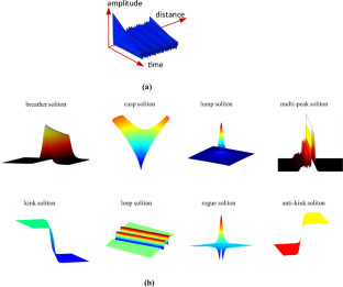
Explore related subjects
- Artificial Intelligence
- Automotive Engineering
Data availability
No datasets were generated or analysed during the current study.
Sutherland, B.: A brief history of the quantum soliton with new results on the quantization of the Toda lattice. Rocky Mt. J. Math. 8 (1/2), 413–428 (1978)
MathSciNet Google Scholar
Geesink, J.H., Meijer, D.K.F.: Bio-soliton model that predicts non-thermal electromagnetic frequency bands, that either stabilize or destabilize living cells. Electromagn. Biol. Med. 36 (4), 357–378 (2017)
Article Google Scholar
Agrawal, G.P.: Nonlinear fiber optics. In: Nonlinear science at the dawn of the 21st Century, pp. 195–211. Springer, Berlin Heidelberg, Berlin, Heidelberg (2000)
Chapter Google Scholar
Geng, K.L., Mou, D.S., Dai, C.Q.: Nondegenerate solitons of 2-coupled mixed derivative nonlinear Schrödinger equations. Nonlinear Dyn. 111 (1), 603–617 (2023)
Yang, Q.F., Ji, Q.X., Wu, L., Shen, B., Wang, H., Bao, C., Vahala, K.: Dispersive-wave-induced noise limits in miniature soliton microwave sources. Nat. Commun. 12 (1), 1442 (2021)
Aksoy, A., Yenikaya, S.: Soliton wave parameter estimation with the help of an artificial neural network by using the experimental data carried out on the nonlinear transmission line. Chaos Solitons Fractals 169 , 113226 (2023)
Article MathSciNet Google Scholar
Ganie, A.H., AlBaidani, M.M., Wazwaz, A.M., Ma, W.X., Shamima, U., Ullah, M.S.: Soliton dynamics and chaotic analysis of the Biswas-Arshed model. Opt. Quant. Electron. 56 (8), 1379 (2024)
Ullah, M.S., Ali, M.Z., Roshid, H.O.: Bifurcation, chaos, and stability analysis to the second fractional WBBM model. PLoS ONE 19 (7), e0307565 (2024)
Alam, N., Ma, W.X., Ullah, M.S., Seadawy, A.R., Akter, M.: Exploration of soliton structures in the Hirota-Maccari system with stability analysis. Mod. Phys. Lett. B (2024). https://doi.org/10.1142/S0217984924504815
Akter, M., Ullah, M.S., Wazwaz, A.M., Seadawy, A.R.: Unveiling Hirota-Maccari model dynamics via diverse elegant methods. Opt. Quant. Electron. 56 (7), 1127 (2024)
Ullah, M.S., Ali, M.Z.: Bifurcation analysis and new waveforms to the fractional KFG equation. Partial Diff. Equ. Appl. Math. 10 , 100716 (2024)
Google Scholar
Ullah, M.S., Ali, M.Z., Roshid, H.O.: Bifurcation analysis and new waveforms to the first fractional WBBM equation. Sci. Rep. 14 (1), 11907 (2024)
Ganie, A.H., Wazwaz, A.M., Seadawy, A.R., Ullah, M.S., Afroz, H.D., Akter, R.: Application of three analytical approaches to the model of ion sound and Langmuir waves. Pramana 98 (2), 46 (2024)
Korteweg, D.J., De Vries, G.: XLI. On the change of form of long waves advancing in a rectangular canal, and on a new type of long stationary waves. Lond., Edinb., Dublin Philos. Mag. J. Sci. 39 (240), 422–443 (1895)
Zabusky, N.J., Kruskal, M.D.: Interaction of" solitons" in a collisionless plasma and the recurrence of initial states. Phys. Rev. Lett. 15 (6), 240 (1965)
Gardner, C.S., Greene, J.M., Kruskal, M.D., Miura, R.M.: Method for solving the Korteweg-deVries equation. Phys. Rev. Lett. 19 (19), 1095 (1967)
Shabat, A., Zakharov, V.: Exact theory of two-dimensional self-focusing and one-dimensional self-modulation of waves in nonlinear media. Sov. Phys. JETP 34 (1), 62 (1972)
Poppenberg, M., Schmitt, K., Wang, Z.Q.: On the existence of soliton solutions to quasilinear Schrödinger equations. Calc. Var. Partial. Differ. Equ. 14 (3), 329–344 (2002)
Hao, R., Li, L., Li, Z., Xue, W., Zhou, G.: A new approach to exact soliton solutions and soliton interaction for the nonlinear Schrödinger equation with variable coefficients. Opt. Commun.Commun. 236 (1–3), 79–86 (2004)
Khalique, C.M., Adeyemo, O.D.: Soliton solutions, travelling wave solutions and conserved quantities for a three-dimensional soliton equation in plasma physics. Commun. Theor. Phys. 73 (12), 125003 (2021)
Nisar, K.S., Ilhan, O.A., Abdulazeez, S.T., Manafian, J., Mohammed, S.A., Osman, M.S.: Novel multiple soliton solutions for some nonlinear PDEs via multiple Exp-function method. Res. Phys. 21 , 103769 (2021)
Guo, R., Hao, H.Q.: Breathers and multi-soliton solutions for the higher-order generalized nonlinear Schrödinger equation. Commun. Nonlinear Sci. Numer. Simul. 18 (9), 2426–2435 (2013)
Yu, W., Liu, W., Zhang, H.: Soliton molecules in the kink, antikink and oscillatory background. Chaos Solitons Fractals 159 , 112132 (2022)
Bisis, S., Ghosh, U., Raut, S.: Construction of fractional granular model and bright, dark, lump, breather types soliton solutions using Hirota bilinear method. Chaos Solitons Fractals 172 , 113520 (2023)
Qiao, Z., Qiao, X.B.: Cusp solitons and cusp-like singular solutions for nonlinear equations. Chaos Solitons Fractals 25 (1), 153–163 (2005)
Luo, X.: Solitons, breathers and rogue waves for the three-component Gross-Pitaevskii equations in the spinor Bose-Einstein condensates. Chaos Solitons Fractals 131 , 109479 (2020)
Nuruzzaman, M., Kumar, D., Inc, M., Uddin, M.A., Alqahtani, R.T.: Localized waves and their novel interaction solutions for a dimensionally reduced (2+ 1)-dimensional Kudryashov Sinelshchikov equation. Res. Phys. 52 , 106786 (2023)
Yao, S.W., Nuruzzaman, M., Kumar, D., Tamanna, N., Inc, M.: Lump solutions to an integrable (3+ 1)-dimensional Boussinesq equation and its dimensionally reduced equations in shallow water. Res. Phys. 45 , 106226 (2023)
Wang, X., Wu, Z., Song, J., Han, W., Yan, Z.: Data-driven soliton solutions and parameters discovery of the coupled nonlinear wave equations via a deep learning method. Chaos Solitons Fractals 180 , 114509 (2024)
Cui, S., Wang, Z., Han, J., Cui, X., Meng, Q.: A deep learning method for solving high-order nonlinear soliton equations. Commun. Theor. Phys. 74 (7), 075007 (2022)
Zhou, Z., Yan, Z.: Deep learning neural networks for the third-order nonlinear Schrödinger equation: bright solitons, breathers, and rogue waves. Commun. Theor. Phys. 73 (10), 105006 (2021)
Zhong, M., Yan, Z.: Data-driven soliton mappings for integrable fractional nonlinear wave equations via deep learning with Fourier neural operator. Chaos Solitons Fractals 165 , 112787 (2022)
Aksoy, A., Yigit, E.: Automatic soliton wave recognition using deep learning algorithms. Chaos Solitons Fractals 174 , 113815 (2023)
Huang, G., Liu, Z., Van Der Maaten, L., Weinberger, K. Q.:Densely connected convolutional networks. In Proceedings of the IEEE conference on computer vision and pattern recognition (pp. 4700–4708). (2017)
Kumar, D., Nuruzzaman, M., Paul, G.C., Hoque, A.: Novel localized waves and interaction solutions for a dimensionally reduced (2+ 1)-dimensional Boussinesq equation from N-soliton solutions. Nonlinear Dyn. 107 (3), 2717–2743 (2022)
Vulli, A., Srinivasu, P.N., Sashank, M.S.K., Shafi, J., Choi, J., Ijaz, M.F.: Fine-tuned DenseNet-169 for breast cancer metastasis prediction using FastAI and 1-cycle policy. Sensors 22 (8), 2988 (2022)
Demir, A., Yilmaz, F., Kose, O.: Early detection of skin cancer using deep learning architectures: resnet-101 and inception-v3. In 2019 medical technologies congress (TIPTEKNO) (pp. 1–4). IEEE. (2019)
Dong, N., Zhao, L., Wu, C.H., Chang, J.F.: Inception v3 based cervical cell classification combined with artificially extracted features. Appl. Soft Comput. 93 , 106311 (2020)
Prusty, S., Patnaik, S., & Dash, S. K.: ResNet50V2: A Transfer Learning Model to Predict Pneumonia with chest X-ray images. In 2022 International Conference on Machine Learning, Computer Systems and Security (MLCSS) (pp. 208–213). IEEE. (2022)
Sailaja, B., VenuGopal, T.: Brain MRI image classification and analysis using modified ResNet50V2 for Parkinson’s disease detection. SN Comput. Sci. 4 (6), 854 (2023)
Raje, N. R., & Jadhav, A.: Automated Diagnosis of Pneumonia through Capsule Network in conjunction with ResNet50v2 model. In 2022 International Conference on Emerging Smart Computing and Informatics (ESCI) (pp. 1–6). IEEE. (2022).
Chabchoub, A., Mozumi, K., Hoffmann, N., Babanin, A.V., Toffoli, A., Steer, J.N., İseda, T.: Directional soliton and breather beams. Proc. Natl. Acad. Sci. 116 (20), 9759–9763 (2019)
Aliyu, A.I., Alshomrani, A.S., Baleanu, D.: Optical solitons for Triki-Bisis equation by two analytic approaches. AIMS Math. 5 (2), 1001–1011 (2020)
Ge, F.F., Tian, S.F.: Mechanisms of nonlinear wave transitions in the (2+ 1)-dimensional generalized breaking soliton equation. Nonlinear Dyn. 105 , 1753–1764 (2021)
Islam, S., Halder, B., Refaie Ali, A.: Optical and rogue type soliton solutions of the (2+ 1) dimensional nonlinear Heisenberg ferromagnetic spin chains equation. Sci. Rep. 13 (1), 9906 (2023)
Nuruzzaman, M., Kumar, D.: Lumps with their some interactions and breathers to an integrable (2+ 1)-dimensional Boussinesq equation in shallow water. Res. Phys. 38 , 105642 (2022)
Zhao, Q., Amin, M.A., Li, X.: Classical Darboux transformation and exact soliton solutions of a two-component complex short pulse equation. AIMS Math. 8 (4), 8811–8828 (2023). https://doi.org/10.3934/math.2023442
Download references
The authors have not disclosed any funding.
Author information
Authors and affiliations.
Department of Electrical-Electronics Engineering, Faculty of Engineering, Bursa Uludag University, Bursa, Turkey
Abdullah Aksoy & Enes Yiğit
You can also search for this author in PubMed Google Scholar
Contributions
Abdullah AKSOY: Conceptualization, Methodology, Software, Investigation, Validation, Resources, Data Arrangement, Visualization, Writing—Review & Editing. Enes YİĞİT: Investigation, Validation, Visualization, Writing—Review & Editing, Oversight.
Corresponding author
Correspondence to Abdullah Aksoy .
Ethics declarations
Conflict of interest.
The authors declare that they have no conflict of interest.
Additional information
Publisher's note.
Springer Nature remains neutral with regard to jurisdictional claims in published maps and institutional affiliations.
Rights and permissions
Springer Nature or its licensor (e.g. a society or other partner) holds exclusive rights to this article under a publishing agreement with the author(s) or other rightsholder(s); author self-archiving of the accepted manuscript version of this article is solely governed by the terms of such publishing agreement and applicable law.
Reprints and permissions
About this article
Aksoy, A., Yiğit, E. Automatic recognition of different 3D soliton wave types using deep learning methods. Nonlinear Dyn (2024). https://doi.org/10.1007/s11071-024-10288-5
Download citation
Received : 10 March 2024
Accepted : 31 August 2024
Published : 09 September 2024
DOI : https://doi.org/10.1007/s11071-024-10288-5
Share this article
Anyone you share the following link with will be able to read this content:
Sorry, a shareable link is not currently available for this article.
Provided by the Springer Nature SharedIt content-sharing initiative
- Soliton wave
- Deep learning algorithm
- Soliton wave types
- Soliton equations
Advertisement
- Find a journal
- Publish with us
- Track your research
IMAGES
VIDEO
COMMENTS
There are many types of data visualization. The most common are scatter plots, line graphs, pie charts, bar charts, heat maps, area charts, choropleth maps and histograms. In this guide, we've put together a list of 33 types of data visualizations. You'll also find an overview of each one and guidelines for when to use them.
1. The Nature of Your Data: The type and structure of your data are key determinants in your choice of visualization. Numerical data might be best served by bar or line charts, while geographical data can be presented as a map. Categorical data, on the other hand, might warrant a pie chart or a treemap. 2.
This type of chart is helpful in quickly identifying whether or not the data is symmetrical or skewed, as well as providing a visual summary of the data set that can be easily interpreted. 7. Waterfall Chart. A waterfall chart is a visual representation that illustrates how a value changes as it's influenced by different factors, such as time ...
6. Scatter Plot. The scatter plot is also among the popular data visualization types and has other names such as a scatter diagram, scatter graph, and correlation chart. Scatter plot helps in many areas of today's world - business, biology, social statistics, data science and etc.
These types of graphs can also help teams assess possible roadblocks because you can analyze data in a tight visual display. For example, I could create a series of bullet graphs measuring performance against benchmarks or use a single bullet graph to visualize these KPIs against their goals: Revenue. Profit. Customer satisfaction. Average ...
The Power of Good Data Visualization. Data visualization involves the use of graphical representations of data, such as graphs, charts, and maps. Compared to descriptive statistics or tables, visuals provide a more effective way to analyze data, including identifying patterns, distributions, and correlations and spotting outliers in complex ...
10. Geographical maps. Source: ubs.com. One of the most versatile types of data visualization is the geographical map, which can bring life to a whole range of different location-specific data. A common example is the distribution of vote share during an election, like that shown in the image.
What is data visualization? Data visualization is the graphical representation of information and data. By using visual elements like charts, graphs, and maps, data visualization tools provide an accessible way to see and understand trends, outliers, and patterns in data.Additionally, it provides an excellent way for employees or business owners to present data to non-technical audiences ...
A histogram is a visual representation of the distribution of data. The graph itself consists of a set of rectangles— each rectangle represents a range of values (called a "bin"), while the height corresponds to the numbers of the data that fall within that range. ... Essentially, any type of content or data that can be broken down into ...
In this article, we will approach the task of choosing a data visualization based on the type of task that you want to perform. Common roles for data visualization include: showing change over time. showing a part-to-whole composition. looking at how data is distributed. comparing values between groups.
Data visualization is the representation of information and data using charts, graphs, maps, and other visual tools. These visualizations allow us to easily understand any patterns, trends, or outliers in a data set. Data visualization also presents data to the general public or specific audiences without technical knowledge in an accessible ...
a visual representation of line chart. A line chart, also known as a line graph, is a visual representation of data points connected by straight lines. One of the most popular data visualization graph types. This chart type is particularly useful for displaying trends and patterns over time, making it an effective choice for time-series data ...
Data visualization is the visual presentation of data or information. The goal of data visualization is to communicate data or information clearly and effectively to readers. Typically, data is visualized in the form of a chart, infographic, diagram or map. The field of data visualization combines both art and data science.
Types of Data Visualization: Charts, Graphs, Infographics, and Dashboards. The diverse landscape of data visualization begins with simple charts and graphs but moves beyond infographics and animated dashboards. Charts, in their various forms - be it bar charts for comparing quantities across categories or line charts depicting trends over ...
Data visualization is the representation of data through use of common graphics, such as charts, plots, infographics and even animations. These visual displays of information communicate complex data relationships and data-driven insights in a way that is easy to understand.
The main goal of data visualization is that it helps unify and bring teams onto the same page. The human mind is wired to grasp visual information more effortlessly than raw data in spreadsheets or detailed reports. Thus, graphical representation of voluminous and intricate data is more user-friendly.
1. Bar Charts. Bar charts are one of the common visualization tool, used to symbolize and compare express facts by way of showing square bars. A bar chart has X and Y Axis where the X Axis represents the types and the Y axis represents the price. The top of the bar represents the price for that class at the y-axis.
2.1: Types of Data Representation. Page ID. Two common types of graphic displays are bar charts and histograms. Both bar charts and histograms use vertical or horizontal bars to represent the number of data points in each category or interval. The main difference graphically is that in a bar chart there are spaces between the bars and in a ...
Here are a handful of different types of data visualization tools that you can begin using right now. 1. Spider Diagrams. Use this template. Spider diagrams, or mind maps, are the master web-weavers of visual representation. They originate from a central concept and extend outwards like a spider's web.
Data Visualization Charts is a method of presenting information and data in a visual way using graphical representation elements like charts, graphs and maps. These visual elements help users easily understand complex datasets quickly and efficiently. There are many different types of visualization charts, each best suited for different data types
6 Real-World Data Visualization Examples. 1. The Most Common Jobs by State. Source: NPR. National Public Radio (NPR) produced a color-coded, interactive display of the most common jobs in each state in each year from 1978 to 2014. By dragging the scroll bar at the bottom of the map, you're able to visualize occupational changes over time.
Another type of data falls in between metric and nominal: ... Instead, solving the example problems in Figure 19 requires that they see the underlying link between the visual and verbal representations of the patterns. This problem arises when visualizations must be linked to text, tables, or mathematical equations. ...
4. Bar Chart. To compare data along two axes, use bar charts. A visual representation of the categories or subjects being measured is shown on one of the axes, which is numerical. 5. Heat Maps. A data visualization method that uses colors to denote values; great for seeing trends in huge datasets. 6.
Color is an important property of the visual world informing behavior. The retinal basis for color vision has been studied in many vertebrate species, including zebrafish, mice, and primates (reviewed in Baden and Osorio, 2019): Signals from different photoreceptor types which are sensitive to different wavelengths are compared by retinal circuits, thereby creating color-opponent cell types.
The overall similarity between the representation of emotions in brain regions and that in visio-linguistic modalities, which involve multi-modal representations of both visual and linguistic ...
2.1 The dataset of soliton wave types. The construction of the dataset involves several distinct phases, as depicted in Fig. 2 Initially, soliton wave types are generated in 3D visual representations via mathematical equations as illustrated in Fig. 2.Each of these examples, along with each specific wave type within the data set, was obtained by solving the corresponding mathematical expressions.