- Skip to secondary menu
- Skip to main content
- Skip to primary sidebar
Statistics By Jim
Making statistics intuitive

Z Test: Uses, Formula & Examples
By Jim Frost Leave a Comment
What is a Z Test?
Use a Z test when you need to compare group means. Use the 1-sample analysis to determine whether a population mean is different from a hypothesized value. Or use the 2-sample version to determine whether two population means differ.
A Z test is a form of inferential statistics . It uses samples to draw conclusions about populations.
For example, use Z tests to assess the following:
- One sample : Do students in an honors program have an average IQ score different than a hypothesized value of 100?
- Two sample : Do two IQ boosting programs have different mean scores?
In this post, learn about when to use a Z test vs T test. Then we’ll review the Z test’s hypotheses, assumptions, interpretation, and formula. Finally, we’ll use the formula in a worked example.
Related post : Difference between Descriptive and Inferential Statistics
Z test vs T test
Z tests and t tests are similar. They both assess the means of one or two groups, have similar assumptions, and allow you to draw the same conclusions about population means.
However, there is one critical difference.
Z tests require you to know the population standard deviation, while t tests use a sample estimate of the standard deviation. Learn more about Population Parameters vs. Sample Statistics .
In practice, analysts rarely use Z tests because it’s rare that they’ll know the population standard deviation. It’s even rarer that they’ll know it and yet need to assess an unknown population mean!
A Z test is often the first hypothesis test students learn because its results are easier to calculate by hand and it builds on the standard normal distribution that they probably already understand. Additionally, students don’t need to know about the degrees of freedom .
Z and T test results converge as the sample size approaches infinity. Indeed, for sample sizes greater than 30, the differences between the two analyses become small.
William Sealy Gosset developed the t test specifically to account for the additional uncertainty associated with smaller samples. Conversely, Z tests are too sensitive to mean differences in smaller samples and can produce statistically significant results incorrectly (i.e., false positives).
When to use a T Test vs Z Test
Let’s put a button on it.
When you know the population standard deviation, use a Z test.
When you have a sample estimate of the standard deviation, which will be the vast majority of the time, the best statistical practice is to use a t test regardless of the sample size.
However, the difference between the two analyses becomes trivial when the sample size exceeds 30.
Learn more about a T-Test Overview: How to Use & Examples and How T-Tests Work .
Z Test Hypotheses
This analysis uses sample data to evaluate hypotheses that refer to population means (µ). The hypotheses depend on whether you’re assessing one or two samples.
One-Sample Z Test Hypotheses
- Null hypothesis (H 0 ): The population mean equals a hypothesized value (µ = µ 0 ).
- Alternative hypothesis (H A ): The population mean DOES NOT equal a hypothesized value (µ ≠ µ 0 ).
When the p-value is less or equal to your significance level (e.g., 0.05), reject the null hypothesis. The difference between your sample mean and the hypothesized value is statistically significant. Your sample data support the notion that the population mean does not equal the hypothesized value.
Related posts : Null Hypothesis: Definition, Rejecting & Examples and Understanding Significance Levels
Two-Sample Z Test Hypotheses
- Null hypothesis (H 0 ): Two population means are equal (µ 1 = µ 2 ).
- Alternative hypothesis (H A ): Two population means are not equal (µ 1 ≠ µ 2 ).
Again, when the p-value is less than or equal to your significance level, reject the null hypothesis. The difference between the two means is statistically significant. Your sample data support the idea that the two population means are different.
These hypotheses are for two-sided analyses. You can use one-sided, directional hypotheses instead. Learn more in my post, One-Tailed and Two-Tailed Hypothesis Tests Explained .
Related posts : How to Interpret P Values and Statistical Significance
Z Test Assumptions
For reliable results, your data should satisfy the following assumptions:
You have a random sample
Drawing a random sample from your target population helps ensure that the sample represents the population. Representative samples are crucial for accurately inferring population properties. The Z test results won’t be valid if your data do not reflect the population.
Related posts : Random Sampling and Representative Samples
Continuous data
Z tests require continuous data . Continuous variables can assume any numeric value, and the scale can be divided meaningfully into smaller increments, such as fractional and decimal values. For example, weight, height, and temperature are continuous.
Other analyses can assess additional data types. For more information, read Comparing Hypothesis Tests for Continuous, Binary, and Count Data .
Your sample data follow a normal distribution, or you have a large sample size
All Z tests assume your data follow a normal distribution . However, due to the central limit theorem, you can ignore this assumption when your sample is large enough.
The following sample size guidelines indicate when normality becomes less of a concern:
- One-Sample : 20 or more observations.
- Two-Sample : At least 15 in each group.
Related posts : Central Limit Theorem and Skewed Distributions
Independent samples
For the two-sample analysis, the groups must contain different sets of items. This analysis compares two distinct samples.
Related post : Independent and Dependent Samples
Population standard deviation is known
As I mention in the Z test vs T test section, use a Z test when you know the population standard deviation. However, when n > 30, the difference between the analyses becomes trivial.
Related post : Standard Deviations
Z Test Formula
These Z test formulas allow you to calculate the test statistic. Use the Z statistic to determine statistical significance by comparing it to the appropriate critical values and use it to find p-values.
The correct formula depends on whether you’re performing a one- or two-sample analysis. Both formulas require sample means (x̅) and sample sizes (n) from your sample. Additionally, you specify the population standard deviation (σ) or variance (σ 2 ), which does not come from your sample.
I present a worked example using the Z test formula at the end of this post.
Learn more about Z-Scores and Test Statistics .
One Sample Z Test Formula

The one sample Z test formula is a ratio.
The numerator is the difference between your sample mean and a hypothesized value for the population mean (µ 0 ). This value is often a strawman argument that you hope to disprove.
The denominator is the standard error of the mean. It represents the uncertainty in how well the sample mean estimates the population mean.
Learn more about the Standard Error of the Mean .
Two Sample Z Test Formula

The two sample Z test formula is also a ratio.
The numerator is the difference between your two sample means.
The denominator calculates the pooled standard error of the mean by combining both samples. In this Z test formula, enter the population variances (σ 2 ) for each sample.
Z Test Critical Values
As I mentioned in the Z vs T test section, a Z test does not use degrees of freedom. It evaluates Z-scores in the context of the standard normal distribution. Unlike the t-distribution , the standard normal distribution doesn’t change shape as the sample size changes. Consequently, the critical values don’t change with the sample size.
To find the critical value for a Z test, you need to know the significance level and whether it is one- or two-tailed.
| 0.01 | Two-Tailed | ±2.576 |
| 0.01 | Left Tail | –2.326 |
| 0.01 | Right Tail | +2.326 |
| 0.05 | Two-Tailed | ±1.960 |
| 0.05 | Left Tail | +1.650 |
| 0.05 | Right Tail | –1.650 |
Learn more about Critical Values: Definition, Finding & Calculator .
Z Test Worked Example
Let’s close this post by calculating the results for a Z test by hand!
Suppose we randomly sampled subjects from an honors program. We want to determine whether their mean IQ score differs from the general population. The general population’s IQ scores are defined as having a mean of 100 and a standard deviation of 15.
We’ll determine whether the difference between our sample mean and the hypothesized population mean of 100 is statistically significant.
Specifically, we’ll use a two-tailed analysis with a significance level of 0.05. Looking at the table above, you’ll see that this Z test has critical values of ± 1.960. Our results are statistically significant if our Z statistic is below –1.960 or above +1.960.
The hypotheses are the following:
- Null (H 0 ): µ = 100
- Alternative (H A ): µ ≠ 100
Entering Our Results into the Formula
Here are the values from our study that we need to enter into the Z test formula:
- IQ score sample mean (x̅): 107
- Sample size (n): 25
- Hypothesized population mean (µ 0 ): 100
- Population standard deviation (σ): 15

The Z-score is 2.333. This value is greater than the critical value of 1.960, making the results statistically significant. Below is a graphical representation of our Z test results showing how the Z statistic falls within the critical region.

We can reject the null and conclude that the mean IQ score for the population of honors students does not equal 100. Based on the sample mean of 107, we know their mean IQ score is higher.
Now let’s find the p-value. We could use technology to do that, such as an online calculator. However, let’s go old school and use a Z table.
To find the p-value that corresponds to a Z-score from a two-tailed analysis, we need to find the negative value of our Z-score (even when it’s positive) and double it.
In the truncated Z-table below, I highlight the cell corresponding to a Z-score of -2.33.

The cell value of 0.00990 represents the area or probability to the left of the Z-score -2.33. We need to double it to include the area > +2.33 to obtain the p-value for a two-tailed analysis.
P-value = 0.00990 * 2 = 0.0198
That p-value is an approximation because it uses a Z-score of 2.33 rather than 2.333. Using an online calculator, the p-value for our Z test is a more precise 0.0196. This p-value is less than our significance level of 0.05, which reconfirms the statistically significant results.
See my full Z-table , which explains how to use it to solve other types of problems.
Share this:

Reader Interactions
Comments and questions cancel reply.
- Practice Mathematical Algorithm
- Mathematical Algorithms
- Pythagorean Triplet
- Fibonacci Number
- Euclidean Algorithm
- LCM of Array
- GCD of Array
- Binomial Coefficient
- Catalan Numbers
- Sieve of Eratosthenes
- Euler Totient Function
- Modular Exponentiation
- Modular Multiplicative Inverse
- Stein's Algorithm
- Juggler Sequence
- Chinese Remainder Theorem
- Quiz on Fibonacci Numbers
Z-test : Formula, Types, Examples
Z-test is especially useful when you have a large sample size and know the population’s standard deviation. Different tests are used in statistics to compare distinct samples or groups and make conclusions about populations. These tests, also referred to as statistical tests, concentrate on examining the probability or possibility of acquiring the observed data under particular premises or hypotheses. They offer a framework for evaluating the evidence for or against a given hypothesis.
Table of Content
What is Z-Test?
Z-test formula, when to use z-test, hypothesis testing, steps to perform z-test, type of z-test, practice problems.

Z-test is a statistical test that is used to determine whether the mean of a sample is significantly different from a known population mean when the population standard deviation is known. It is particularly useful when the sample size is large (>30).
Z-test can also be defined as a statistical method that is used to determine whether the distribution of the test statistics can be approximated using the normal distribution or not. It is the method to determine whether two sample means are approximately the same or different when their variance is known and the sample size is large (should be >= 30).
The Z-test compares the difference between the sample mean and the population means by considering the standard deviation of the sampling distribution. The resulting Z-score represents the number of standard deviations that the sample mean deviates from the population mean. This Z-Score is also known as Z-Statistics, and can be formulated as:
[Tex]\text{Z-Score} = \frac{\bar{x}-\mu}{\sigma} [/Tex]
- [Tex]\bar{x} [/Tex] : mean of the sample.
- [Tex]\mu [/Tex] : mean of the population.
- [Tex]\sigma [/Tex] : Standard deviation of the population.
z-test assumes that the test statistic (z-score) follows a standard normal distribution.
The average family annual income in India is 200k, with a standard deviation of 5k, and the average family annual income in Delhi is 300k.
Then Z-Score for Delhi will be.
[Tex]\begin{aligned} \text{Z-Score}&=\frac{\bar{x}-\mu}{\sigma} \\&=\frac{300-200}{5} \\&=20 \end{aligned} [/Tex]
This indicates that the average family’s annual income in Delhi is 20 standard deviations above the mean of the population (India).
- The sample size should be greater than 30. Otherwise, we should use the t-test.
- Samples should be drawn at random from the population.
- The standard deviation of the population should be known.
- Samples that are drawn from the population should be independent of each other.
- The data should be normally distributed , however, for a large sample size, it is assumed to have a normal distribution because central limit theorem
A hypothesis is an educated guess/claim about a particular property of an object. Hypothesis testing is a way to validate the claim of an experiment.
- Null Hypothesis: The null hypothesis is a statement that the value of a population parameter (such as proportion, mean, or standard deviation) is equal to some claimed value. We either reject or fail to reject the null hypothesis. The null hypothesis is denoted by H 0 .
- Alternate Hypothesis: The alternative hypothesis is the statement that the parameter has a value that is different from the claimed value. It is denoted by H A .
- Level of significance: It means the degree of significance in which we accept or reject the null hypothesis. Since in most of the experiments 100% accuracy is not possible for accepting or rejecting a hypothesis, we, therefore, select a level of significance. It is denoted by alpha (∝).
- First, identify the null and alternate hypotheses.
- Determine the level of significance (∝).
- Find the critical value of z in the z-test using
- n: sample size.
- Now compare with the hypothesis and decide whether to reject or not reject the null hypothesis
Left-tailed Test
In this test, our region of rejection is located to the extreme left of the distribution. Here our null hypothesis is that the claimed value is less than or equal to the mean population value.

Right-tailed Test
In this test, our region of rejection is located to the extreme right of the distribution. Here our null hypothesis is that the claimed value is less than or equal to the mean population value.

One-Tailed Test
A school claimed that the students who study that are more intelligent than the average school. On calculating the IQ scores of 50 students, the average turns out to be 110. The mean of the population IQ is 100 and the standard deviation is 15. State whether the claim of the principal is right or not at a 5% significance level.
- First, we define the null hypothesis and the alternate hypothesis. Our null hypothesis will be: [Tex]H_0 : \mu = 100 [/Tex] and our alternate hypothesis. [Tex]H_A : \mu > 100 [/Tex]
- State the level of significance. Here, our level of significance is given in this question ( [Tex]\alpha [/Tex] =0.05), if not given then we take ∝=0.05 in general.
- Now, we compute the Z-Score: X = 110 Mean = 100 Standard Deviation = 15 Number of samples = 50 [Tex]\begin{aligned} \text{Z-Score}&=\frac{\bar{x}-\mu}{\sigma/\sqrt{n}} \\&=\frac{110-100}{15/\sqrt{50}} \\&=\frac{10}{2.12} \\&=4.71 \end{aligned} [/Tex]
- Now, we look up to the z-table. For the value of ∝=0.05, the z-score for the right-tailed test is 1.645.
- Here 4.71 >1.645, so we reject the null hypothesis.
- If the z-test statistics are less than the z-score, then we will not reject the null hypothesis.
Code Implementations of One-Tailed Z-Test
# Import the necessary libraries import numpy as np import scipy.stats as stats # Given information sample_mean = 110 population_mean = 100 population_std = 15 sample_size = 50 alpha = 0.05 # compute the z-score z_score = ( sample_mean - population_mean ) / ( population_std / np . sqrt ( 50 )) print ( 'Z-Score :' , z_score ) # Approach 1: Using Critical Z-Score # Critical Z-Score z_critical = stats . norm . ppf ( 1 - alpha ) print ( 'Critical Z-Score :' , z_critical ) # Hypothesis if z_score > z_critical : print ( "Reject Null Hypothesis" ) else : print ( "Fail to Reject Null Hypothesis" ) # Approach 2: Using P-value # P-Value : Probability of getting less than a Z-score p_value = 1 - stats . norm . cdf ( z_score ) print ( 'p-value :' , p_value ) # Hypothesis if p_value < alpha : print ( "Reject Null Hypothesis" ) else : print ( "Fail to Reject Null Hypothesis" )
Z-Score : 4.714045207910317Critical Z-Score : 1.6448536269514722Reject Null Hypothesisp-value : 1.2142337364462463e-06Reject Null Hypothesis
Two-tailed test
In this test, our region of rejection is located to both extremes of the distribution. Here our null hypothesis is that the claimed value is equal to the mean population value.

Below is an example of performing the z-test:
Two-sampled z-test
In this test, we have provided 2 normally distributed and independent populations, and we have drawn samples at random from both populations. Here, we consider u 1 and u 2 to be the population mean, and X 1 and X 2 to be the observed sample mean. Here, our null hypothesis could be like this:
[Tex]H_{0} : \mu_{1} -\mu_{2} = 0 [/Tex]
and alternative hypothesis
[Tex]H_{1} : \mu_{1} – \mu_{2} \ne 0 [/Tex]
and the formula for calculating the z-test score:
[Tex]Z = \frac{\left ( \overline{X_{1}} – \overline{X_{2}} \right ) – \left ( \mu_{1} – \mu_{2} \right )}{\sqrt{\frac{\sigma_{1}^2}{n_{1}} + \frac{\sigma_{2}^2}{n_{2}}}} [/Tex]
where [Tex]\sigma_1 [/Tex] and [Tex]\sigma_2 [/Tex] are the standard deviation and n 1 and n 2 are the sample size of population corresponding to u 1 and u 2 .
There are two groups of students preparing for a competition: Group A and Group B. Group A has studied offline classes, while Group B has studied online classes. After the examination, the score of each student comes. Now we want to determine whether the online or offline classes are better.
Group A: Sample size = 50, Sample mean = 75, Sample standard deviation = 10 Group B: Sample size = 60, Sample mean = 80, Sample standard deviation = 12
Assuming a 5% significance level, perform a two-sample z-test to determine if there is a significant difference between the online and offline classes.
Step 1: Null & Alternate Hypothesis
- Null Hypothesis: There is no significant difference between the mean score between the online and offline classes [Tex] \mu_1 -\mu_2 = 0 [/Tex]
- Alternate Hypothesis: There is a significant difference in the mean scores between the online and offline classes. [Tex] \mu_1 -\mu_2 \neq 0 [/Tex]
Step 2: Significance Label
- Significance Label: 5% [Tex]\alpha = 0.05 [/Tex]
Step 3: Z-Score
[Tex]\begin{aligned} \text{Z-score} &= \frac{(x_1-x_2)-(\mu_1 -\mu_2)} {\sqrt{\frac{\sigma_1^2}{n_1}+\frac{\sigma_2^2}{n_1}}} \\ &= \frac{(75-80)-0} {\sqrt{\frac{10^2}{50}+\frac{12^2}{60}}} \\ &= \frac{-5} {\sqrt{2+2.4}} \\ &= \frac{-5} {2.0976} \\&=-2.384 \end{aligned} [/Tex]
Step 4: Check to Critical Z-Score value in the Z-Table for apha/2 = 0.025
- Critical Z-Score = 1.96
Step 5: Compare with the absolute Z-Score value
- absolute(Z-Score) > Critical Z-Score
- Reject the null hypothesis. There is a significant difference between the online and offline classes.
Code Implementations on Two-sampled Z-test
import numpy as np import scipy.stats as stats # Group A (Offline Classes) n1 = 50 x1 = 75 s1 = 10 # Group B (Online Classes) n2 = 60 x2 = 80 s2 = 12 # Null Hypothesis = mu_1-mu_2 = 0 # Hypothesized difference (under the null hypothesis) D = 0 # Set the significance level alpha = 0.05 # Calculate the test statistic (z-score) z_score = (( x1 - x2 ) - D ) / np . sqrt (( s1 ** 2 / n1 ) + ( s2 ** 2 / n2 )) print ( 'Z-Score:' , np . abs ( z_score )) # Calculate the critical value z_critical = stats . norm . ppf ( 1 - alpha / 2 ) print ( 'Critical Z-Score:' , z_critical ) # Compare the test statistic with the critical value if np . abs ( z_score ) > z_critical : print ( """Reject the null hypothesis. There is a significant difference between the online and offline classes.""" ) else : print ( """Fail to reject the null hypothesis. There is not enough evidence to suggest a significant difference between the online and offline classes.""" ) # Approach 2: Using P-value # P-Value : Probability of getting less than a Z-score p_value = 2 * ( 1 - stats . norm . cdf ( np . abs ( z_score ))) print ( 'P-Value :' , p_value ) # Compare the p-value with the significance level if p_value < alpha : print ( """Reject the null hypothesis. There is a significant difference between the online and offline classes.""" ) else : print ( """Fail to reject the null hypothesis. There is not enough evidence to suggest significant difference between the online and offline classes.""" )
Z-Score: 2.3836564731139807 Critical Z-Score: 1.959963984540054 Reject the null hypothesis. There is a significant difference between the online and offline classes. P-Value : 0.01714159544079563 Reject the null hypothesis. There is a significant difference between the online and offline classes.
Solved examples :
Example 1: One-sample Z-test
Problem: A company claims that the average battery life of their new smartphone is 12 hours. A consumer group tests 100 phones and finds the average battery life to be 11.8 hours with a population standard deviation of 0.5 hours. At a 5% significance level, is there evidence to refute the company’s claim?
Solution: Step 1: State the hypotheses H₀: μ = 12 (null hypothesis) H₁: μ ≠ 12 (alternative hypothesis) Step 2: Calculate the Z-score Z = (x̄ – μ) / (σ / √n) = (11.8 – 12) / (0.5 / √100) = -0.2 / 0.05 = -4 Step 3: Find the critical value (two-tailed test at 5% significance) Z₀.₀₂₅ = ±1.96 Step 4: Compare Z-score with critical value |-4| > 1.96, so we reject the null hypothesis. Conclusion: There is sufficient evidence to refute the company’s claim about battery life.
Problem: A researcher wants to compare the effectiveness of two different medications for reducing blood pressure. Medication A is tested on 50 patients, resulting in a mean reduction of 15 mmHg with a standard deviation of 3 mmHg. Medication B is tested on 60 patients, resulting in a mean reduction of 13 mmHg with a standard deviation of 4 mmHg. At a 1% significance level, is there a significant difference between the two medications?
Step 1: State the hypotheses H₀: μ₁ – μ₂ = 0 (null hypothesis) H₁: μ₁ – μ₂ ≠ 0 (alternative hypothesis) Step 2: Calculate the Z-score Z = (x̄₁ – x̄₂) / √((σ₁²/n₁) + (σ₂²/n₂)) = (15 – 13) / √((3²/50) + (4²/60)) = 2 / √(0.18 + 0.2667) = 2 / 0.6455 = 3.10 Step 3: Find the critical value (two-tailed test at 1% significance) Z₀.₀₀₅ = ±2.576 Step 4: Compare Z-score with critical value 3.10 > 2.576, so we reject the null hypothesis. Conclusion: There is a significant difference between the effectiveness of the two medications at the 1% significance level.
Problem 3 : A polling company claims that 60% of voters support a new policy. In a sample of 1000 voters, 570 support the policy. At a 5% significance level, is there evidence to support the company’s claim?
Step 1: State the hypotheses H₀: p = 0.60 (null hypothesis) H₁: p ≠ 0.60 (alternative hypothesis) Step 2: Calculate the Z-score p̂ = 570/1000 = 0.57 (sample proportion) Z = (p̂ – p) / √(p(1-p)/n) = (0.57 – 0.60) / √(0.60(1-0.60)/1000) = -0.03 / √(0.24/1000) = -0.03 / 0.0155 = -1.94 Step 3: Find the critical value (two-tailed test at 5% significance) Z₀.₀₂₅ = ±1.96 Step 4: Compare Z-score with critical value |-1.94| < 1.96, so we fail to reject the null hypothesis. Conclusion: There is not enough evidence to refute the polling company’s claim at the 5% significance level.
Problem 4 : A manufacturer claims that their light bulbs last an average of 1000 hours. A sample of 100 bulbs has a mean life of 985 hours. The population standard deviation is known to be 50 hours. At a 5% significance level, is there evidence to reject the manufacturer’s claim?
Solution: H₀: μ = 1000 H₁: μ ≠ 1000 Z = (x̄ – μ) / (σ / √n) = (985 – 1000) / (50 / √100) = -15 / 5 = -3 Critical value (α = 0.05, two-tailed): ±1.96 |-3| > 1.96, so reject H₀. Conclusion: There is sufficient evidence to reject the manufacturer’s claim at the 5% significance level.
Example 5 : Two factories produce semiconductors. Factory A’s chips have a mean resistance of 100 ohms with a standard deviation of 5 ohms. Factory B’s chips have a mean resistance of 98 ohms with a standard deviation of 4 ohms. Samples of 50 chips from each factory are tested. At a 1% significance level, is there a difference in mean resistance between the two factories?
H₀: μA – μB = 0 H₁: μA – μB ≠ 0 Z = (x̄A – x̄B) / √((σA²/nA) + (σB²/nB)) = (100 – 98) / √((5²/50) + (4²/50)) = 2 / √(0.5 + 0.32) = 2 / 0.872 = 2.29 Critical value (α = 0.01, two-tailed): ±2.576 |2.29| < 2.576, so fail to reject H₀. Conclusion: There is not enough evidence to conclude a difference in mean resistance at the 1% significance level.
Problem 6 : A political analyst claims that 40% of voters in a certain district support a new tax policy. In a random sample of 500 voters, 220 support the policy. At a 5% significance level, is there evidence to reject the analyst’s claim?
H₀: p = 0.40 H₁: p ≠ 0.40 p̂ = 220/500 = 0.44 Z = (p̂ – p) / √(p(1-p)/n) = (0.44 – 0.40) / √(0.40(1-0.40)/500) = 0.04 / 0.0219 = 1.83 Critical value (α = 0.05, two-tailed): ±1.96 |1.83| < 1.96, so fail to reject H₀. Conclusion: There is not enough evidence to reject the analyst’s claim at the 5% significance level.
Problem 7 : Two advertising methods are compared. Method A results in 150 sales out of 1000 contacts. Method B results in 180 sales out of 1200 contacts. At a 5% significance level, is there a difference in the effectiveness of the two methods?
H₀: pA – pB = 0 H₁: pA – pB ≠ 0 p̂A = 150/1000 = 0.15 p̂B = 180/1200 = 0.15 p̂ = (150 + 180) / (1000 + 1200) = 0.15 Z = (p̂A – p̂B) / √(p̂(1-p̂)(1/nA + 1/nB)) = (0.15 – 0.15) / √(0.15(1-0.15)(1/1000 + 1/1200)) = 0 / 0.0149 = 0 Critical value (α = 0.05, two-tailed): ±1.96 |0| < 1.96, so fail to reject H₀. Conclusion: There is no significant difference in the effectiveness of the two advertising methods at the 5% significance level.
Problem 8 : A new treatment for a disease is tested in two cities. In City A, 120 out of 400 patients recover. In City B, 140 out of 500 patients recover. At a 5% significance level, is there a difference in the recovery rates between the two cities?
H₀: pA – pB = 0 H₁: pA – pB ≠ 0 p̂A = 120/400 = 0.30 p̂B = 140/500 = 0.28 p̂ = (120 + 140) / (400 + 500) = 0.2889 Z = (p̂A – p̂B) / √(p̂(1-p̂)(1/nA + 1/nB)) = (0.30 – 0.28) / √(0.2889(1-0.2889)(1/400 + 1/500)) = 0.02 / 0.0316 = 0.633 Critical value (α = 0.05, two-tailed): ±1.96 |0.633| < 1.96, so fail to reject H₀. Conclusion: There is not enough evidence to conclude a difference in recovery rates between the two cities at the 5% significance level.
Problem 9 : Two advertising methods are compared. Method A results in 150 sales out of 1000 contacts. Method B results in 180 sales out of 1200 contacts. At a 5% significance level, is there a difference in the effectiveness of the two methods?
Problem 10 : A company claims that their product weighs 500 grams on average. A sample of 64 products has a mean weight of 498 grams. The population standard deviation is known to be 8 grams. At a 1% significance level, is there evidence to reject the company’s claim?
H₀: μ = 500 H₁: μ ≠ 500 Z = (x̄ – μ) / (σ / √n) = (498 – 500) / (8 / √64) = -2 / 1 = -2 Critical value (α = 0.01, two-tailed): ±2.576 |-2| < 2.576, so fail to reject H₀. Conclusion: There is not enough evidence to reject the company’s claim at the 1% significance level.
1).A cereal company claims that their boxes contain an average of 350 grams of cereal. A consumer group tests 100 boxes and finds a mean weight of 345 grams with a known population standard deviation of 15 grams. At a 5% significance level, is there evidence to refute the company’s claim?
2).A study compares the effect of two different diets on cholesterol levels. Diet A is tested on 50 people, resulting in a mean reduction of 25 mg/dL with a standard deviation of 8 mg/dL. Diet B is tested on 60 people, resulting in a mean reduction of 22 mg/dL with a standard deviation of 7 mg/dL. At a 1% significance level, is there a significant difference between the two diets?
3).A politician claims that 60% of voters in her district support her re-election. In a random sample of 1000 voters, 570 support her. At a 5% significance level, is there evidence to reject the politician’s claim?
4).Two different teaching methods are compared. Method A results in 80 students passing out of 120 students. Method B results in 90 students passing out of 150 students. At a 5% significance level, is there a difference in the effectiveness of the two methods?
5).A company claims that their new energy-saving light bulbs last an average of 10,000 hours. A sample of 64 bulbs has a mean life of 9,800 hours. The population standard deviation is known to be 500 hours. At a 1% significance level, is there evidence to reject the company’s claim?
6).The mean salary of employees in a large corporation is said to be $75,000 per year. A union representative suspects this is too high and surveys 100 randomly selected employees, finding a mean salary of $72,500. The population standard deviation is known to be $8,000. At a 5% significance level, is there evidence to support the union representative’s suspicion?
7).Two factories produce computer chips. Factory A’s chips have a mean processing speed of 3.2 GHz with a standard deviation of 0.2 GHz. Factory B’s chips have a mean processing speed of 3.3 GHz with a standard deviation of 0.25 GHz. Samples of 100 chips from each factory are tested. At a 5% significance level, is there a difference in mean processing speed between the two factories?
8).A new vaccine is claimed to be 90% effective. In a clinical trial with 500 participants, 440 develop immunity. At a 1% significance level, is there evidence to reject the claim about the vaccine’s effectiveness?
9).Two different advertising campaigns are tested. Campaign A results in 250 sales out of 2000 views. Campaign B results in 300 sales out of 2500 views. At a 5% significance level, is there a difference in the effectiveness of the two campaigns?
10).A quality control manager claims that the defect rate in a production line is 5%. In a sample of 1000 items, 65 are found to be defective. At a 5% significance level, is there evidence to suggest that the actual defect rate is different from the claimed 5%?
Type 1 error and Type II error
- Type I error: Type 1 error has occurred when we reject the null hypothesis, even when the hypothesis is true. This error is denoted by alpha.
- Type II error: Type II error occurred when we didn’t reject the null hypothesis, even when the hypothesis is false. This error is denoted by beta.
| Null Hypothesis is TRUE | Null Hypothesis is FALSE | |
|---|---|---|
| Reject Null Hypothesis | Type I Error (False Positive) | Correct decision |
| Fail to Reject the Null Hypothesis | Correct decision | Type II error (False Negative) |
Z-tests are used to determine whether there is a statistically significant difference between a sample statistic and a population parameter, or between two population parameters.Z-tests are statistical tools used to determine if there’s a significant difference between a sample statistic and a population parameter, or between two population parameters. They’re applicable when dealing with large sample sizes (typically n > 30) and known population standard deviations. Z-tests can be used for analyzing means or proportions in both one-sample and two-sample scenarios. The process involves stating hypotheses, calculating a Z-score, comparing it to a critical value based on the chosen significance level (often 5% or 1%), and then making a decision to reject or fail to reject the null hypothesis.
What is the main limitation of the z-test?
The limitation of Z-Tests is that we don’t usually know the population standard deviation. What we do is: When we don’t know the population’s variability, we assume that the sample’s variability is a good basis for estimating the population’s variability.
What is the minimum sample for z-test?
A z-test can only be used if the population standard deviation is known and the sample size is 30 data points or larger. Otherwise, a t-test should be employed.
What is the application of z-test?
It is also used to determine if there is a significant difference between the mean of two independent samples. The z-test can also be used to compare the population proportion to an assumed proportion or to determine the difference between the population proportion of two samples.
What is the theory of the z-test?
The z test is a commonly used hypothesis test in inferential statistics that allows us to compare two populations using the mean values of samples from those populations, or to compare the mean of one population to a hypothesized value, when what we are interested in comparing is a continuous variable.
Please Login to comment...
Similar reads.
- Engineering Mathematics
- Machine Learning
- Mathematical
- Best Twitch Extensions for 2024: Top Tools for Viewers and Streamers
- Discord Emojis List 2024: Copy and Paste
- Best Adblockers for Twitch TV: Enjoy Ad-Free Streaming in 2024
- PS4 vs. PS5: Which PlayStation Should You Buy in 2024?
- 15 Most Important Aptitude Topics For Placements [2024]
Improve your Coding Skills with Practice
What kind of Experience do you want to share?
Z test is a statistical test that is conducted on data that approximately follows a normal distribution. The z test can be performed on one sample, two samples, or on proportions for hypothesis testing. It checks if the means of two large samples are different or not when the population variance is known.
A z test can further be classified into left-tailed, right-tailed, and two-tailed hypothesis tests depending upon the parameters of the data. In this article, we will learn more about the z test, its formula, the z test statistic, and how to perform the test for different types of data using examples.
| 1. | |
| 2. | |
| 3. | |
| 4. | |
| 5. | |
| 6. |
What is Z Test?
A z test is a test that is used to check if the means of two populations are different or not provided the data follows a normal distribution. For this purpose, the null hypothesis and the alternative hypothesis must be set up and the value of the z test statistic must be calculated. The decision criterion is based on the z critical value.
Z Test Definition
A z test is conducted on a population that follows a normal distribution with independent data points and has a sample size that is greater than or equal to 30. It is used to check whether the means of two populations are equal to each other when the population variance is known. The null hypothesis of a z test can be rejected if the z test statistic is statistically significant when compared with the critical value.
Z Test Formula
The z test formula compares the z statistic with the z critical value to test whether there is a difference in the means of two populations. In hypothesis testing , the z critical value divides the distribution graph into the acceptance and the rejection regions. If the test statistic falls in the rejection region then the null hypothesis can be rejected otherwise it cannot be rejected. The z test formula to set up the required hypothesis tests for a one sample and a two-sample z test are given below.
One-Sample Z Test
A one-sample z test is used to check if there is a difference between the sample mean and the population mean when the population standard deviation is known. The formula for the z test statistic is given as follows:
z = \(\frac{\overline{x}-\mu}{\frac{\sigma}{\sqrt{n}}}\). \(\overline{x}\) is the sample mean, \(\mu\) is the population mean, \(\sigma\) is the population standard deviation and n is the sample size.
The algorithm to set a one sample z test based on the z test statistic is given as follows:
Left Tailed Test:
Null Hypothesis: \(H_{0}\) : \(\mu = \mu_{0}\)
Alternate Hypothesis: \(H_{1}\) : \(\mu < \mu_{0}\)
Decision Criteria: If the z statistic < z critical value then reject the null hypothesis.
Right Tailed Test:
Alternate Hypothesis: \(H_{1}\) : \(\mu > \mu_{0}\)
Decision Criteria: If the z statistic > z critical value then reject the null hypothesis.
Two Tailed Test:
Alternate Hypothesis: \(H_{1}\) : \(\mu \neq \mu_{0}\)
Two Sample Z Test
A two sample z test is used to check if there is a difference between the means of two samples. The z test statistic formula is given as follows:
z = \(\frac{(\overline{x_{1}}-\overline{x_{2}})-(\mu_{1}-\mu_{2})}{\sqrt{\frac{\sigma_{1}^{2}}{n_{1}}+\frac{\sigma_{2}^{2}}{n_{2}}}}\). \(\overline{x_{1}}\), \(\mu_{1}\), \(\sigma_{1}^{2}\) are the sample mean, population mean and population variance respectively for the first sample. \(\overline{x_{2}}\), \(\mu_{2}\), \(\sigma_{2}^{2}\) are the sample mean, population mean and population variance respectively for the second sample.
The two-sample z test can be set up in the same way as the one-sample test. However, this test will be used to compare the means of the two samples. For example, the null hypothesis is given as \(H_{0}\) : \(\mu_{1} = \mu_{2}\).

Z Test for Proportions
A z test for proportions is used to check the difference in proportions. A z test can either be used for one proportion or two proportions. The formulas are given as follows.
One Proportion Z Test
A one proportion z test is used when there are two groups and compares the value of an observed proportion to a theoretical one. The z test statistic for a one proportion z test is given as follows:
z = \(\frac{p-p_{0}}{\sqrt{\frac{p_{0}(1-p_{0})}{n}}}\). Here, p is the observed value of the proportion, \(p_{0}\) is the theoretical proportion value and n is the sample size.
The null hypothesis is that the two proportions are the same while the alternative hypothesis is that they are not the same.
Two Proportion Z Test
A two proportion z test is conducted on two proportions to check if they are the same or not. The test statistic formula is given as follows:
z =\(\frac{p_{1}-p_{2}-0}{\sqrt{p(1-p)\left ( \frac{1}{n_{1}} +\frac{1}{n_{2}}\right )}}\)
where p = \(\frac{x_{1}+x_{2}}{n_{1}+n_{2}}\)
\(p_{1}\) is the proportion of sample 1 with sample size \(n_{1}\) and \(x_{1}\) number of trials.
\(p_{2}\) is the proportion of sample 2 with sample size \(n_{2}\) and \(x_{2}\) number of trials.
How to Calculate Z Test Statistic?
The most important step in calculating the z test statistic is to interpret the problem correctly. It is necessary to determine which tailed test needs to be conducted and what type of test does the z statistic belong to. Suppose a teacher claims that his section's students will score higher than his colleague's section. The mean score is 22.1 for 60 students belonging to his section with a standard deviation of 4.8. For his colleague's section, the mean score is 18.8 for 40 students and the standard deviation is 8.1. Test his claim at \(\alpha\) = 0.05. The steps to calculate the z test statistic are as follows:
- Identify the type of test. In this example, the means of two populations have to be compared in one direction thus, the test is a right-tailed two-sample z test.
- Set up the hypotheses. \(H_{0}\): \(\mu_{1} = \mu_{2}\), \(H_{1}\): \(\mu_{1} > \mu_{2}\).
- Find the critical value at the given alpha level using the z table. The critical value is 1.645.
- Determine the z test statistic using the appropriate formula. This is given by z = \(\frac{(\overline{x_{1}}-\overline{x_{2}})-(\mu_{1}-\mu_{2})}{\sqrt{\frac{\sigma_{1}^{2}}{n_{1}}+\frac{\sigma_{2}^{2}}{n_{2}}}}\). Substitute values in this equation. \(\overline{x_{1}}\) = 22.1, \(\sigma_{1}\) = 4.8, \(n_{1}\) = 60, \(\overline{x_{2}}\) = 18.8, \(\sigma_{2}\) = 8.1, \(n_{2}\) = 40 and \(\mu_{1} - \mu_{2} = 0\). Thus, z = 2.32
- Compare the critical value and test statistic to arrive at a conclusion. As 2.32 > 1.645 thus, the null hypothesis can be rejected. It can be concluded that there is enough evidence to support the teacher's claim that the scores of students are better in his class.
Z Test vs T-Test
Both z test and t-test are univariate tests used on the means of two datasets. The differences between both tests are outlined in the table given below:
| Z Test | T-Test |
|---|---|
| A z test is a statistical test that is used to check if the means of two data sets are different when the population variance is known. | A is used to check if the means of two data sets are different when the population variance is not known. |
| The sample size is greater than or equal to 30. | The sample size is lesser than 30. |
| The follows a normal distribution. | The data follows a student-t distribution. |
| The one-sample z test statistic is given by \(\frac{\overline{x}-\mu}{\frac{\sigma}{\sqrt{n}}}\) | The t test statistic is given as \(\frac{\overline{x}-\mu}{\frac{s}{\sqrt{n}}}\) where s is the sample standard deviation |
Related Articles:
- Probability and Statistics
- Data Handling
- Summary Statistics
Important Notes on Z Test
- Z test is a statistical test that is conducted on normally distributed data to check if there is a difference in means of two data sets.
- The sample size should be greater than 30 and the population variance must be known to perform a z test.
- The one-sample z test checks if there is a difference in the sample and population mean,
- The two sample z test checks if the means of two different groups are equal.
Examples on Z Test
Example 1: A teacher claims that the mean score of students in his class is greater than 82 with a standard deviation of 20. If a sample of 81 students was selected with a mean score of 90 then check if there is enough evidence to support this claim at a 0.05 significance level.
Solution: As the sample size is 81 and population standard deviation is known, this is an example of a right-tailed one-sample z test.
\(H_{0}\) : \(\mu = 82\)
\(H_{1}\) : \(\mu > 82\)
From the z table the critical value at \(\alpha\) = 1.645
z = \(\frac{\overline{x}-\mu}{\frac{\sigma}{\sqrt{n}}}\)
\(\overline{x}\) = 90, \(\mu\) = 82, n = 81, \(\sigma\) = 20
As 3.6 > 1.645 thus, the null hypothesis is rejected and it is concluded that there is enough evidence to support the teacher's claim.
Answer: Reject the null hypothesis
Example 2: An online medicine shop claims that the mean delivery time for medicines is less than 120 minutes with a standard deviation of 30 minutes. Is there enough evidence to support this claim at a 0.05 significance level if 49 orders were examined with a mean of 100 minutes?
Solution: As the sample size is 49 and population standard deviation is known, this is an example of a left-tailed one-sample z test.
\(H_{0}\) : \(\mu = 120\)
\(H_{1}\) : \(\mu < 120\)
From the z table the critical value at \(\alpha\) = -1.645. A negative sign is used as this is a left tailed test.
\(\overline{x}\) = 100, \(\mu\) = 120, n = 49, \(\sigma\) = 30
As -4.66 < -1.645 thus, the null hypothesis is rejected and it is concluded that there is enough evidence to support the medicine shop's claim.
Example 3: A company wants to improve the quality of products by reducing defects and monitoring the efficiency of assembly lines. In assembly line A, there were 18 defects reported out of 200 samples while in line B, 25 defects out of 600 samples were noted. Is there a difference in the procedures at a 0.05 alpha level?
Solution: This is an example of a two-tailed two proportion z test.
\(H_{0}\): The two proportions are the same.
\(H_{1}\): The two proportions are not the same.
As this is a two-tailed test the alpha level needs to be divided by 2 to get 0.025.
Using this, the critical value from the z table is 1.96.
\(n_{1}\) = 200, \(n_{2}\) = 600
\(p_{1}\) = 18 / 200 = 0.09
\(p_{2}\) = 25 / 600 = 0.0416
p = (18 + 25) / (200 + 600) = 0.0537
z =\(\frac{p_{1}-p_{2}-0}{\sqrt{p(1-p)\left ( \frac{1}{n_{1}} +\frac{1}{n_{2}}\right )}}\) = 2.62
As 2.62 > 1.96 thus, the null hypothesis is rejected and it is concluded that there is a significant difference between the two lines.
go to slide go to slide go to slide

Book a Free Trial Class
FAQs on Z Test
What is a z test in statistics.
A z test in statistics is conducted on data that is normally distributed to test if the means of two datasets are equal. It can be performed when the sample size is greater than 30 and the population variance is known.
What is a One-Sample Z Test?
A one-sample z test is used when the population standard deviation is known, to compare the sample mean and the population mean. The z test statistic is given by the formula \(\frac{\overline{x}-\mu}{\frac{\sigma}{\sqrt{n}}}\).
What is the Two-Sample Z Test Formula?
The two sample z test is used when the means of two populations have to be compared. The z test formula is given as \(\frac{(\overline{x_{1}}-\overline{x_{2}})-(\mu_{1}-\mu_{2})}{\sqrt{\frac{\sigma_{1}^{2}}{n_{1}}+\frac{\sigma_{2}^{2}}{n_{2}}}}\).
What is a One Proportion Z test?
A one proportion z test is used to check if the value of the observed proportion is different from the value of the theoretical proportion. The z statistic is given by \(\frac{p-p_{0}}{\sqrt{\frac{p_{0}(1-p_{0})}{n}}}\).
What is a Two Proportion Z Test?
When the proportions of two samples have to be compared then the two proportion z test is used. The formula is given by \(\frac{p_{1}-p_{2}-0}{\sqrt{p(1-p)\left ( \frac{1}{n_{1}} +\frac{1}{n_{2}}\right )}}\).
How Do You Find the Z Test?
The steps to perform the z test are as follows:
- Set up the null and alternative hypotheses.
- Find the critical value using the alpha level and z table.
- Calculate the z statistic.
- Compare the critical value and the test statistic to decide whether to reject or not to reject the null hypothesis.
What is the Difference Between the Z Test and the T-Test?
A z test is used on large samples n ≥ 30 and normally distributed data while a t-test is used on small samples (n < 30) following a student t distribution . Both tests are used to check if the means of two datasets are the same.
Z-test Calculator
Table of contents
This Z-test calculator is a tool that helps you perform a one-sample Z-test on the population's mean . Two forms of this test - a two-tailed Z-test and a one-tailed Z-tests - exist, and can be used depending on your needs. You can also choose whether the calculator should determine the p-value from Z-test or you'd rather use the critical value approach!
Read on to learn more about Z-test in statistics, and, in particular, when to use Z-tests, what is the Z-test formula, and whether to use Z-test vs. t-test. As a bonus, we give some step-by-step examples of how to perform Z-tests!
Or you may also check our t-statistic calculator , where you can learn the concept of another essential statistic. If you are also interested in F-test, check our F-statistic calculator .
What is a Z-test?
A one sample Z-test is one of the most popular location tests. The null hypothesis is that the population mean value is equal to a given number, μ 0 \mu_0 μ 0 :
We perform a two-tailed Z-test if we want to test whether the population mean is not μ 0 \mu_0 μ 0 :
and a one-tailed Z-test if we want to test whether the population mean is less/greater than μ 0 \mu_0 μ 0 :
Let us now discuss the assumptions of a one-sample Z-test.
When do I use Z-tests?
You may use a Z-test if your sample consists of independent data points and:
the data is normally distributed , and you know the population variance ;
the sample is large , and data follows a distribution which has a finite mean and variance. You don't need to know the population variance.
The reason these two possibilities exist is that we want the test statistics that follow the standard normal distribution N ( 0 , 1 ) \mathrm N(0, 1) N ( 0 , 1 ) . In the former case, it is an exact standard normal distribution, while in the latter, it is approximately so, thanks to the central limit theorem.
The question remains, "When is my sample considered large?" Well, there's no universal criterion. In general, the more data points you have, the better the approximation works. Statistics textbooks recommend having no fewer than 50 data points, while 30 is considered the bare minimum.
Z-test formula
Let x 1 , . . . , x n x_1, ..., x_n x 1 , ... , x n be an independent sample following the normal distribution N ( μ , σ 2 ) \mathrm N(\mu, \sigma^2) N ( μ , σ 2 ) , i.e., with a mean equal to μ \mu μ , and variance equal to σ 2 \sigma ^2 σ 2 .
We pose the null hypothesis, H 0 : μ = μ 0 \mathrm H_0 \!\!:\!\! \mu = \mu_0 H 0 : μ = μ 0 .
We define the test statistic, Z , as:
x ˉ \bar x x ˉ is the sample mean, i.e., x ˉ = ( x 1 + . . . + x n ) / n \bar x = (x_1 + ... + x_n) / n x ˉ = ( x 1 + ... + x n ) / n ;
μ 0 \mu_0 μ 0 is the mean postulated in H 0 \mathrm H_0 H 0 ;
n n n is sample size; and
σ \sigma σ is the population standard deviation.
In what follows, the uppercase Z Z Z stands for the test statistic (treated as a random variable), while the lowercase z z z will denote an actual value of Z Z Z , computed for a given sample drawn from N(μ,σ²).
If H 0 \mathrm H_0 H 0 holds, then the sum S n = x 1 + . . . + x n S_n = x_1 + ... + x_n S n = x 1 + ... + x n follows the normal distribution, with mean n μ 0 n \mu_0 n μ 0 and variance n 2 σ n^2 \sigma n 2 σ . As Z Z Z is the standardization (z-score) of S n / n S_n/n S n / n , we can conclude that the test statistic Z Z Z follows the standard normal distribution N ( 0 , 1 ) \mathrm N(0, 1) N ( 0 , 1 ) , provided that H 0 \mathrm H_0 H 0 is true. By the way, we have the z-score calculator if you want to focus on this value alone.
If our data does not follow a normal distribution, or if the population standard deviation is unknown (and thus in the formula for Z Z Z we substitute the population standard deviation σ \sigma σ with sample standard deviation), then the test statistics Z Z Z is not necessarily normal. However, if the sample is sufficiently large, then the central limit theorem guarantees that Z Z Z is approximately N ( 0 , 1 ) \mathrm N(0, 1) N ( 0 , 1 ) .
In the sections below, we will explain to you how to use the value of the test statistic, z z z , to make a decision , whether or not you should reject the null hypothesis . Two approaches can be used in order to arrive at that decision: the p-value approach, and critical value approach - and we cover both of them! Which one should you use? In the past, the critical value approach was more popular because it was difficult to calculate p-value from Z-test. However, with help of modern computers, we can do it fairly easily, and with decent precision. In general, you are strongly advised to report the p-value of your tests!
p-value from Z-test
Formally, the p-value is the smallest level of significance at which the null hypothesis could be rejected. More intuitively, p-value answers the questions: provided that I live in a world where the null hypothesis holds, how probable is it that the value of the test statistic will be at least as extreme as the z z z - value I've got for my sample? Hence, a small p-value means that your result is very improbable under the null hypothesis, and so there is strong evidence against the null hypothesis - the smaller the p-value, the stronger the evidence.
To find the p-value, you have to calculate the probability that the test statistic, Z Z Z , is at least as extreme as the value we've actually observed, z z z , provided that the null hypothesis is true. (The probability of an event calculated under the assumption that H 0 \mathrm H_0 H 0 is true will be denoted as P r ( event ∣ H 0 ) \small \mathrm{Pr}(\text{event} | \mathrm{H_0}) Pr ( event ∣ H 0 ) .) It is the alternative hypothesis which determines what more extreme means :
- Two-tailed Z-test: extreme values are those whose absolute value exceeds ∣ z ∣ |z| ∣ z ∣ , so those smaller than − ∣ z ∣ -|z| − ∣ z ∣ or greater than ∣ z ∣ |z| ∣ z ∣ . Therefore, we have:
The symmetry of the normal distribution gives:
- Left-tailed Z-test: extreme values are those smaller than z z z , so
- Right-tailed Z-test: extreme values are those greater than z z z , so
To compute these probabilities, we can use the cumulative distribution function, (cdf) of N ( 0 , 1 ) \mathrm N(0, 1) N ( 0 , 1 ) , which for a real number, x x x , is defined as:
Also, p-values can be nicely depicted as the area under the probability density function (pdf) of N ( 0 , 1 ) \mathrm N(0, 1) N ( 0 , 1 ) , due to:
Two-tailed Z-test and one-tailed Z-test
With all the knowledge you've got from the previous section, you're ready to learn about Z-tests.
- Two-tailed Z-test:
From the fact that Φ ( − z ) = 1 − Φ ( z ) \Phi(-z) = 1 - \Phi(z) Φ ( − z ) = 1 − Φ ( z ) , we deduce that
The p-value is the area under the probability distribution function (pdf) both to the left of − ∣ z ∣ -|z| − ∣ z ∣ , and to the right of ∣ z ∣ |z| ∣ z ∣ :

- Left-tailed Z-test:
The p-value is the area under the pdf to the left of our z z z :

- Right-tailed Z-test:
The p-value is the area under the pdf to the right of z z z :

The decision as to whether or not you should reject the null hypothesis can be now made at any significance level, α \alpha α , you desire!
if the p-value is less than, or equal to, α \alpha α , the null hypothesis is rejected at this significance level; and
if the p-value is greater than α \alpha α , then there is not enough evidence to reject the null hypothesis at this significance level.
Z-test critical values & critical regions
The critical value approach involves comparing the value of the test statistic obtained for our sample, z z z , to the so-called critical values . These values constitute the boundaries of regions where the test statistic is highly improbable to lie . Those regions are often referred to as the critical regions , or rejection regions . The decision of whether or not you should reject the null hypothesis is then based on whether or not our z z z belongs to the critical region.
The critical regions depend on a significance level, α \alpha α , of the test, and on the alternative hypothesis. The choice of α \alpha α is arbitrary; in practice, the values of 0.1, 0.05, or 0.01 are most commonly used as α \alpha α .
Once we agree on the value of α \alpha α , we can easily determine the critical regions of the Z-test:
To decide the fate of H 0 \mathrm H_0 H 0 , check whether or not your z z z falls in the critical region:
If yes, then reject H 0 \mathrm H_0 H 0 and accept H 1 \mathrm H_1 H 1 ; and
If no, then there is not enough evidence to reject H 0 \mathrm H_0 H 0 .
As you see, the formulae for the critical values of Z-tests involve the inverse, Φ − 1 \Phi^{-1} Φ − 1 , of the cumulative distribution function (cdf) of N ( 0 , 1 ) \mathrm N(0, 1) N ( 0 , 1 ) .
How to use the one-sample Z-test calculator?
Our calculator reduces all the complicated steps:
Choose the alternative hypothesis: two-tailed or left/right-tailed.
In our Z-test calculator, you can decide whether to use the p-value or critical regions approach. In the latter case, set the significance level, α \alpha α .
Enter the value of the test statistic, z z z . If you don't know it, then you can enter some data that will allow us to calculate your z z z for you:
- sample mean x ˉ \bar x x ˉ (If you have raw data, go to the average calculator to determine the mean);
- tested mean μ 0 \mu_0 μ 0 ;
- sample size n n n ; and
- population standard deviation σ \sigma σ (or sample standard deviation if your sample is large).
Results appear immediately below the calculator.
If you want to find z z z based on p-value , please remember that in the case of two-tailed tests there are two possible values of z z z : one positive and one negative, and they are opposite numbers. This Z-test calculator returns the positive value in such a case. In order to find the other possible value of z z z for a given p-value, just take the number opposite to the value of z z z displayed by the calculator.
Z-test examples
To make sure that you've fully understood the essence of Z-test, let's go through some examples:
- A bottle filling machine follows a normal distribution. Its standard deviation, as declared by the manufacturer, is equal to 30 ml. A juice seller claims that the volume poured in each bottle is, on average, one liter, i.e., 1000 ml, but we suspect that in fact the average volume is smaller than that...
Formally, the hypotheses that we set are the following:
H 0 : μ = 1000 ml \mathrm H_0 \! : \mu = 1000 \text{ ml} H 0 : μ = 1000 ml
H 1 : μ < 1000 ml \mathrm H_1 \! : \mu \lt 1000 \text{ ml} H 1 : μ < 1000 ml
We went to a shop and bought a sample of 9 bottles. After carefully measuring the volume of juice in each bottle, we've obtained the following sample (in milliliters):
1020 , 970 , 1000 , 980 , 1010 , 930 , 950 , 980 , 980 \small 1020, 970, 1000, 980, 1010, 930, 950, 980, 980 1020 , 970 , 1000 , 980 , 1010 , 930 , 950 , 980 , 980 .
Sample size: n = 9 n = 9 n = 9 ;
Sample mean: x ˉ = 980 m l \bar x = 980 \ \mathrm{ml} x ˉ = 980 ml ;
Population standard deviation: σ = 30 m l \sigma = 30 \ \mathrm{ml} σ = 30 ml ;
And, therefore, p-value = Φ ( − 2 ) ≈ 0.0228 \text{p-value} = \Phi(-2) \approx 0.0228 p-value = Φ ( − 2 ) ≈ 0.0228 .
As 0.0228 < 0.05 0.0228 \lt 0.05 0.0228 < 0.05 , we conclude that our suspicions aren't groundless; at the most common significance level, 0.05, we would reject the producer's claim, H 0 \mathrm H_0 H 0 , and accept the alternative hypothesis, H 1 \mathrm H_1 H 1 .
We tossed a coin 50 times. We got 20 tails and 30 heads. Is there sufficient evidence to claim that the coin is biased?
Clearly, our data follows Bernoulli distribution, with some success probability p p p and variance σ 2 = p ( 1 − p ) \sigma^2 = p (1-p) σ 2 = p ( 1 − p ) . However, the sample is large, so we can safely perform a Z-test. We adopt the convention that getting tails is a success.
Let us state the null and alternative hypotheses:
H 0 : p = 0.5 \mathrm H_0 \! : p = 0.5 H 0 : p = 0.5 (the coin is fair - the probability of tails is 0.5 0.5 0.5 )
H 1 : p ≠ 0.5 \mathrm H_1 \! : p \ne 0.5 H 1 : p = 0.5 (the coin is biased - the probability of tails differs from 0.5 0.5 0.5 )
In our sample we have 20 successes (denoted by ones) and 30 failures (denoted by zeros), so:
Sample size n = 50 n = 50 n = 50 ;
Sample mean x ˉ = 20 / 50 = 0.4 \bar x = 20/50 = 0.4 x ˉ = 20/50 = 0.4 ;
Population standard deviation is given by σ = 0.5 × 0.5 \sigma = \sqrt{0.5 \times 0.5} σ = 0.5 × 0.5 (because 0.5 0.5 0.5 is the proportion p p p hypothesized in H 0 \mathrm H_0 H 0 ). Hence, σ = 0.5 \sigma = 0.5 σ = 0.5 ;
- And, therefore
Since 0.1573 > 0.1 0.1573 \gt 0.1 0.1573 > 0.1 we don't have enough evidence to reject the claim that the coin is fair , even at such a large significance level as 0.1 0.1 0.1 . In that case, you may safely toss it to your Witcher or use the coin flip probability calculator to find your chances of getting, e.g., 10 heads in a row (which are extremely low!).
What is the difference between Z-test vs t-test?
We use a t-test for testing the population mean of a normally distributed dataset which had an unknown population standard deviation . We get this by replacing the population standard deviation in the Z-test statistic formula by the sample standard deviation, which means that this new test statistic follows (provided that H₀ holds) the t-Student distribution with n-1 degrees of freedom instead of N(0,1) .
When should I use t-test over the Z-test?
For large samples, the t-Student distribution with n degrees of freedom approaches the N(0,1). Hence, as long as there are a sufficient number of data points (at least 30), it does not really matter whether you use the Z-test or the t-test, since the results will be almost identical. However, for small samples with unknown variance, remember to use the t-test instead of Z-test .
How do I calculate the Z test statistic?
To calculate the Z test statistic:
- Compute the arithmetic mean of your sample .
- From this mean subtract the mean postulated in null hypothesis .
- Multiply by the square root of size sample .
- Divide by the population standard deviation .
- That's it, you've just computed the Z test statistic!
Here, we perform a Z-test for population mean μ. Null hypothesis H₀: μ = μ₀.
Alternative hypothesis H₁
Significance level α
The probability that we reject the true hypothesis H₀ (type I error).
Z Test: Definition & Two Proportion Z-Test
What is a z test.

For example, if someone said they had found a new drug that cures cancer, you would want to be sure it was probably true. A hypothesis test will tell you if it’s probably true, or probably not true. A Z test, is used when your data is approximately normally distributed (i.e. the data has the shape of a bell curve when you graph it).
When you can run a Z Test.
Several different types of tests are used in statistics (i.e. f test , chi square test , t test ). You would use a Z test if:
- Your sample size is greater than 30 . Otherwise, use a t test .
- Data points should be independent from each other. In other words, one data point isn’t related or doesn’t affect another data point.
- Your data should be normally distributed . However, for large sample sizes (over 30) this doesn’t always matter.
- Your data should be randomly selected from a population, where each item has an equal chance of being selected.
- Sample sizes should be equal if at all possible.
How do I run a Z Test?
Running a Z test on your data requires five steps:
- State the null hypothesis and alternate hypothesis .
- Choose an alpha level .
- Find the critical value of z in a z table .
- Calculate the z test statistic (see below).
- Compare the test statistic to the critical z value and decide if you should support or reject the null hypothesis .
You could perform all these steps by hand. For example, you could find a critical value by hand , or calculate a z value by hand . For a step by step example, watch the following video: Watch the video for an example:

Can’t see the video? Click here to watch it on YouTube. You could also use technology, for example:
- Two sample z test in Excel .
- Find a critical z value on the TI 83 .
- Find a critical value on the TI 89 (left-tail) .
Two Proportion Z-Test
Watch the video to see a two proportion z-test:
Can’t see the video? Click here to watch it on YouTube.
A Two Proportion Z-Test (or Z-interval) allows you to calculate the true difference in proportions of two independent groups to a given confidence interval .
There are a few familiar conditions that need to be met for the Two Proportion Z-Interval to be valid.
- The groups must be independent. Subjects can be in one group or the other, but not both – like teens and adults.
- The data must be selected randomly and independently from a homogenous population. A survey is a common example.
- The population should be at least ten times bigger than the sample size. If the population is teenagers for example, there should be at least ten times as many total teenagers as the number of teenagers being surveyed.
- The null hypothesis (H 0 ) for the test is that the proportions are the same.
- The alternate hypothesis (H 1 ) is that the proportions are not the same.
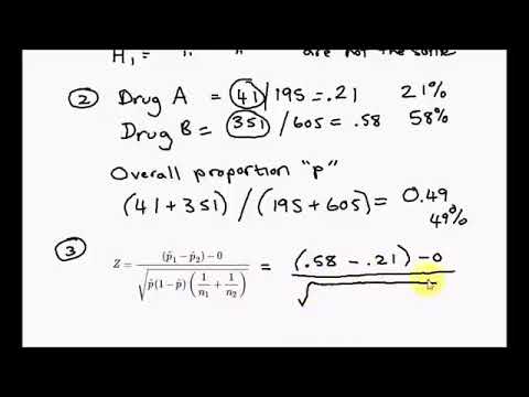
Example question: let’s say you’re testing two flu drugs A and B. Drug A works on 41 people out of a sample of 195. Drug B works on 351 people in a sample of 605. Are the two drugs comparable? Use a 5% alpha level .
Step 1: Find the two proportions:
- P 1 = 41/195 = 0.21 (that’s 21%)
- P 2 = 351/605 = 0.58 (that’s 58%).
Set these numbers aside for a moment.
Step 2: Find the overall sample proportion . The numerator will be the total number of “positive” results for the two samples and the denominator is the total number of people in the two samples.
- p = (41 + 351) / (195 + 605) = 0.49.
Set this number aside for a moment.

Solving the formula, we get: Z = 8.99
We need to find out if the z-score falls into the “ rejection region .”

Step 5: Compare the calculated z-score from Step 3 with the table z-score from Step 4. If the calculated z-score is larger, you can reject the null hypothesis.
8.99 > 1.96, so we can reject the null hypothesis .
Example 2: Suppose that in a survey of 700 women and 700 men, 35% of women and 30% of men indicated that they support a particular presidential candidate. Let’s say we wanted to find the true difference in proportions of these two groups to a 95% confidence interval .
At first glance the survey indicates that women support the candidate more than men by about 5% . However, for this statistical inference to be valid we need to construct a range of values to a given confidence interval.
To do this, we use the formula for Two Proportion Z-Interval:

Plugging in values we find the true difference in proportions to be

Based on the results of the survey, we are 95% confident that the difference in proportions of women and men that support the presidential candidate is between about 0 % and 10% .
Check out our YouTube channel for more stats help and tips!
Z-Test for Statistical Hypothesis Testing Explained
The Z-test is a statistical hypothesis test that determines where the distribution of the statistic we are measuring, like the mean, is part of the normal distribution.
The Z-test is a statistical hypothesis test used to determine where the distribution of the test statistic we are measuring, like the mean , is part of the normal distribution .
There are multiple types of Z-tests, however, we’ll focus on the easiest and most well known one, the one sample mean test. This is used to determine if the difference between the mean of a sample and the mean of a population is statistically significant.
What Is a Z-Test?
A Z-test is a type of statistical hypothesis test where the test-statistic follows a normal distribution.
The name Z-test comes from the Z-score of the normal distribution. This is a measure of how many standard deviations away a raw score or sample statistics is from the populations’ mean.
Z-tests are the most common statistical tests conducted in fields such as healthcare and data science . Therefore, it’s an essential concept to understand.
Requirements for a Z-Test
In order to conduct a Z-test, your statistics need to meet a few requirements, including:
- A Sample size that’s greater than 30. This is because we want to ensure our sample mean comes from a distribution that is normal. As stated by the c entral limit theorem , any distribution can be approximated as normally distributed if it contains more than 30 data points.
- The standard deviation and mean of the population is known .
- The sample data is collected/acquired randomly .
More on Data Science: What Is Bootstrapping Statistics?
Z-Test Steps
There are four steps to complete a Z-test. Let’s examine each one.
4 Steps to a Z-Test
- State the null hypothesis.
- State the alternate hypothesis.
- Choose your critical value.
- Calculate your Z-test statistics.
1. State the Null Hypothesis
The first step in a Z-test is to state the null hypothesis, H_0 . This what you believe to be true from the population, which could be the mean of the population, μ_0 :
2. State the Alternate Hypothesis
Next, state the alternate hypothesis, H_1 . This is what you observe from your sample. If the sample mean is different from the population’s mean, then we say the mean is not equal to μ_0:
3. Choose Your Critical Value
Then, choose your critical value, α , which determines whether you accept or reject the null hypothesis. Typically for a Z-test we would use a statistical significance of 5 percent which is z = +/- 1.96 standard deviations from the population’s mean in the normal distribution:
This critical value is based on confidence intervals.
4. Calculate Your Z-Test Statistic
Compute the Z-test Statistic using the sample mean, μ_1 , the population mean, μ_0 , the number of data points in the sample, n and the population’s standard deviation, σ :
If the test statistic is greater (or lower depending on the test we are conducting) than the critical value, then the alternate hypothesis is true because the sample’s mean is statistically significant enough from the population mean.
Another way to think about this is if the sample mean is so far away from the population mean, the alternate hypothesis has to be true or the sample is a complete anomaly.
More on Data Science: Basic Probability Theory and Statistics Terms to Know
Z-Test Example
Let’s go through an example to fully understand the one-sample mean Z-test.
A school says that its pupils are, on average, smarter than other schools. It takes a sample of 50 students whose average IQ measures to be 110. The population, or the rest of the schools, has an average IQ of 100 and standard deviation of 20. Is the school’s claim correct?
The null and alternate hypotheses are:
Where we are saying that our sample, the school, has a higher mean IQ than the population mean.
Now, this is what’s called a right-sided, one-tailed test as our sample mean is greater than the population’s mean. So, choosing a critical value of 5 percent, which equals a Z-score of 1.96 , we can only reject the null hypothesis if our Z-test statistic is greater than 1.96.
If the school claimed its students’ IQs were an average of 90, then we would use a left-tailed test, as shown in the figure above. We would then only reject the null hypothesis if our Z-test statistic is less than -1.96.
Computing our Z-test statistic, we see:
Therefore, we have sufficient evidence to reject the null hypothesis, and the school’s claim is right.
Hope you enjoyed this article on Z-tests. In this post, we only addressed the most simple case, the one-sample mean test. However, there are other types of tests, but they all follow the same process just with some small nuances.
Recent Data Science Articles

One-sample Z-test: Hypothesis Testing, Effect Size, and Power
Ke (kay) fang ( [email protected] ).
Hey, I’m Kay! This guide provides an introduction to the fundamental concepts of and relationships between hypothesis testing, effect size, and power analysis, using the one-sample z-test as a prime example. While the primary goal is to elucidate the idea behind hypothesis testing, this guide does try to carefully derive the math details behind the test in the hope that it helps clarification. DISCLAIMER: It’s important to mention that the one-sample z-test is rarely used due to its restrictive assumptions. As such, there are limited resources on the subject, compelling me to derive most of the formulas, particularly those related to power, on my own. This self-reliance might increase the likelihood of errors. If you detect any inaccuracies or inconsistencies, please don’t hesitate to let me know, and I’ll make the necessary updates. Happy learning! ;)
Single sample Z-test
I. the data generating process.
In a single sample z-test, our data generating process (DGP) assumes that our observations of a random variable \(X\) are independently drawn from one identical distribution (i.i.d.) with mean \(\mu\) and variance \(\sigma^2\) .
Important Notation:
Here we use the capital \(\bar{X}\) to denote the sample mean to refer it as a random variable. And the \(X_i\) refer to each element in a sample also as a random variable.
Later, when we have an actual observed sample, we would use the lower case letter \(x_i\) to denote each observation/realization of the random variable \(X_i\) and calculate the observed sample mean \(\bar{x}\) and treat it as an realization of our sample mean \(\bar{X}\) .
The sample mean is defined as below. As indicated in previous guide, the sample mean is an unbiased estimator of population expectation under i.i.d. assumption.
\[\bar{X} = \frac{\sum^n_i X_i}{n}\]
The expectation of the sample mean should be:
\[ \begin{align*} E(\bar{X}) =& E(\frac{1}{n} \cdot \sum^n_i(X_i)) \\ =& \frac{1}{n} \cdot \sum^n_iE(X_i)\\ =&\frac{1}{n}\cdot n \cdot \mu\\ =& \mu \end{align*} \]
and the variance of the sample mean would be:
\[ \begin{align*} Var(\bar{X}) =& Var(\frac{1}{n} \cdot \sum^n_i(X_i))\\ =& \frac{1}{n^2} \cdot \sum^n_i Var(X_i)\\ =&\frac{1}{n^2} \cdot n \cdot \sigma^2\\ =& \frac{\sigma^2}{n}\\[2ex] *\text{Note: } & Var(X_1 +X_2) = Var(X_1) + Var(X_2) + Cov(X_1, X_2)\\ &\text{As the samples are drawn individually, } Cov(X_1, X_2) =0, \\ &Var(X_1 +X_2) = Var(X_1) + Var(X_2)\\ \end{align*} \]
More importantly, according to The Central Limit Theorem (CLT), even we did not specify the original distribution of \(x\) , if the original distributions of \(x\) have finite variances, as n become sufficiently large (rule of thumb: n >30), the distribution of \(\bar{x}\) become a normal distribution:
\[\bar{X} \sim N(\mu, \frac{\sigma^2}{n})\]
Given the nature of the normal distribution, we know the probability density function of \(\bar{X}\) would be
\[f_{pdf}(\bar{X}|\mu, \sigma, n) = \frac{1}{\left(\frac{\sigma}{\sqrt{n}}\right)\sqrt{2\pi}} \cdot \exp\left[-\frac{(\bar{X}-\mu)^2}{2 \cdot \left(\frac{\sigma^2}{n}\right)}\right]\]
This can be tedious to calculate so we could standardize the normal distribution to a standard normal distribution ( \(N(0, 1)\) ).
\[ Z = (\frac{\bar{X} - \mu}{\sigma/\sqrt{n}}) = (\frac{\sqrt{n} \cdot (\bar{X} - \mu)}{\sigma})\sim N(0, 1)\\ \]
Important Notation: Similar to \(\bar{X}\) and \(\bar{x}\) , we use \(Z\) to refer to the random variable and \(z\) to refer to the observation from a fixed sample.
Also we could get the theoretical probability of getting Z between an interval from the distribution by
\[ Pr(z_{min} < Z < z_{max}) = \Phi(z_{max}) - \Phi(z_{min})\\[2ex] \text{where } \Phi(k) = \int^k_{-\infty} f_{pdf}(Z|\mu, \sigma,n)\ dZ\\[2ex] f_{pdf}(Z|\mu, \sigma,n) = \frac{1}{\sqrt{2\pi}} \cdot exp(-\frac{1}{2}Z^2)\\[2ex] Z|\mu, \sigma,n = \frac{\sqrt{n} \cdot (\bar{X} - \mu)}{\sigma} \]
II. The Hypothesis Testing
1. logic of hypothesis testing: the null hypothesis.
For a one-sample Z-test, we assume we know the variance parameter \(\sigma^2\) of our data generating distribution (a very unrealistic assumption, but let’s stick with it for now)
Given a sample, we could also know the sample size n, the observed sample mean \(\bar{x}\) (remember we use lower case so it don’t get confused as we view the sample mean \(\bar{X}\) as a random variable in our DGP).
The aim of our hypothesis testing is then, given our knowledge about the \(\sigma\) , n and the \(\bar{x}\) , we can test hypothesis about our sample mean \(\mu\) . Specifically, the null hypothesis ( \(H_0\) ) stating that,
\(\mu = \mu_{H_0}\) (a two-tailed test)
\(\mu \geq \mu_{H_0}\) (a right-tailed test)
\(\mu \leq \mu_{H_0}\) (a left-tailed test)
We make this decision follow the logic that: if, given the null hypothesis is true, the probability of getting a sample mean \(\bar{X}\) (or its corresponding test statistics \(Z\) ) that is as extreme or more extreme as the observed sample mean \(\bar{x}\) (or its corresponding test statistics \(z\) ) is smaller than some threshold ( \(\alpha\) ), we would rather believe the null hypothesis is not true.
The p-value represents the probability of observing a test statistic \(Z = \frac{\sqrt{n} \cdot (\bar{X} - \mu_0)}{\sigma}\) as extreme as, or more extreme than, the one computed from the sample \(z = \frac{\sqrt{n} \cdot (\bar{x} - \mu_0)}{\sigma}\) , given that the null hypothesis is true.
The threshold we set is called significance level, denoted as \(\alpha\) . As we reject the null if the p-value is below \(\alpha\) , this also means that we have the probability of \(\alpha\) to falsely reject the null given our null is true and our observed case is indeed extreme (known as Type I error).
Moreover, given the distribution under the null, the \(\alpha\) correspond to a specific value(s) of z called the critical value(s), which we can denote as \(z_c\) .
There are two practical ways we could conduct this hypothesis testing (they are actually the same), we could either calculate the p-value and compare them to the \(\alpha\) , or compare the test statistics \(z\) with the critical value \(z_c\) .
2. Calculation of p-value
Two-tail test: p-value.
If we are concerned with the probability that our actual \(\mu\) is different (either larger or smaller) than \(\mu_{H_0}\) , we are doing a two-tail test .
For a two-tailed test, when we refer to values that are “as extreme or more extreme” than the observed test statistic, we’re considering deviations in both positive and negative directions from zero.
- Specifically, if \(z\) is positive, the p-value encompasses the probability of getting a \(Z\) that is greater than or equal to \(z\) and the probability of observing a z-value less than or equal to \(-z\) .
Therefore, the two-tailed p-value is:
\[ \begin{align*} \text{If}\ z > 0\ \text{and } & \text{alternative hypo: }\ \mu\neq \mu_{H_0}, \\[2ex] p\text{-value} =& P(Z > z) + P(Z < -z)\\ =& (1 - \Phi(z)) + \Phi(-z) =\int^{\infty}_{z} f_{pdf}(Z)\ dZ + \int^{-z}_{-\infty} f_{pdf}(Z)\ dZ,\\[2ex] & \text{As the distribution is symmetrical to 0}\\[2ex] =& 2 \cdot P(Z > z) = 2 \cdot (1-\Phi(z)) = 2 \cdot \int^{\infty}_{z}f(Z)dZ\\[2ex] =& 2 \cdot P(Z < -z) = 2 \cdot \Phi(-z)= 2 \cdot \int^{-z}_{-\infty}f(Z)dZ\\[2ex] & \text{In abosolute sense: }\\[2ex] =& 2 \cdot P(Z > |z|) = 2 \cdot (1-\Phi(|z|)) = 2 \cdot \int^{\infty}_{|z|}f(Z)dZ\\[2ex] z = &\frac{\sqrt{n} \cdot (\bar{x} - \mu_0)}{\sigma}\ \text{is calculated from the observed sample} \end{align*} \]
- Conversely, if \(z\) is negative, we consider values less than or equal to \(z\) and those greater than or equal to \(-z\) .
\[ \begin{align*} \text{If}\ z < 0\ \text{and } & \text{alternative hypo: }\ \mu\neq \mu_{H_0}, \\[2ex] p\text{-value} =& P(Z < z) + P(Z > -z) = \Phi(z) + (1-\Phi(-z))=\int^{z}_{-\infty} f_{pdf}(Z)\ dZ + \int^{\infty}_{-z} f_{pdf}(Z)\ dZ,\\[2ex] & \text{As the distribution is symmetrical to 0}\\[2ex] =& 2 \cdot P(Z < z) = 2 \cdot \Phi(z) = 2 \cdot \int^{z}_{-\infty}f(Z)dZ\\[2ex] =& 2 \cdot P(Z > -z) = 2 \cdot (1-\Phi(-z)) =2 \cdot \int^{\infty}_{-z}f(Z)dZ\\[2ex] & \text{In abosolute sense: }\\[2ex] =& 2 \cdot P(Z > |z|) = 2 \cdot (1-\Phi(|z|)) =2 \cdot \int^{\infty}_{|z|}f(Z)dZ\\[2ex] z = &\frac{\sqrt{n} \cdot (\bar{x} - \mu_0)}{\sigma}\ \text{is calculated from the observed sample} \end{align*} \]
- Overall, we can combine these two scenarios by using the absolute value of \(z\) .
\[ \text{Overall, for two-tailed test, alternative hypo: } \mu\neq \mu_{H_0}\\[2ex] p\text{-value} = 2 \cdot P(Z > |z|) = 2 \cdot (1-\Phi(|z|)) = 2 \cdot \int^{\infty}_{|z|}f_{pdf}(Z)dZ,\\[2ex] z = \frac{\sqrt{n} \cdot (\bar{x} - \mu_0)}{\sigma}\ \text{is calculated from the observed sample} \]
One-tail test: p-value
And if we are only concerned with the probability that our actual \(\mu\) is larger (or smaller) than \(\mu_{H_0}\) , we are doing a one-tail test .
For a one-tailed test, when we refer to values that are “as extreme or more extreme” than the observed test statistic, we’re considering deviations only in one direction from zero.
Therefore, the one-tailed p-value is:
\[ p-value= \begin{cases} P(Z > z) = 1 - \Phi(z)=\int^{\infty}_{z} f_{pdf}(Z)\ dZ,\quad \text{alternative hypo: } \mu> \mu_{H_0}\\[2ex] P(Z < z) = \Phi(z)= \int^{z}_{-\infty} f_{pdf}(Z)\ dZ, \quad \text{alternative hypo: } \mu < \mu_{H_0}\\[2ex] \end{cases} \\[2ex] z = \frac{\sqrt{n} \cdot (\bar{x} - \mu_0)}{\sigma}\ \text{is calculated from the observed sample} \]
If the p-value is smaller than our significance level \(\alpha\) , we can reject the null.
\[p-value(z) < \alpha \Rightarrow \text{reject } H_0: \mu = \mu_{H_0}\]
3. Critical value and rejection area
Alternatively, we could choose to not to calculate p-value for our observed \(z\) , but compare our \(z\) to the z value(s) corresponding to our \(\alpha\) .
Two-tailed test
Under a two-tailed test, we use:
\[ Pr(Z > |z|) < \frac{1}{2}\alpha \]
The critical value \(z_{\alpha/2}\) is defined as:
\[ z_{\alpha/2}= arg_{z_i} \Big[Pr(Z > z_{i}) = \frac{ \alpha}{2} \Big] = \Phi^{-1} \Big(1 -\frac{ \alpha}{2} \Big) \]
Due to the symmetry of the standard normal distribution:
\[ -z_{\alpha/2} = arg_{z_i} \Big[Pr(Z < -z_{i}) = \frac{ \alpha}{2} \Big] =\Phi^{-1} \Big(\frac{ \alpha}{2} \Big) \]
Our decision rule then implies:
\[ |z| > z_{\alpha/2},\ \text{if alternative hypo: } \mu \neq \mu_{H_0} \]
One-tailed test
Similarly for one-tailed test, the critical value \(z_{c}\) is:
\[ z_{\alpha} = \begin{cases} arg_{z_i}[Pr(Z > z_{i}) = \alpha] = \Phi^{-1}(1-\alpha), & \text{if alternative hypo: } \mu> \mu_{H_0}\\[2ex] arg_{z_i}[Pr(Z < z_{i}) = \alpha] = \Phi^{-1}(\alpha), & \text{if alternative hypo: } \mu < \mu_{H_0}\\[2ex] \end{cases} \]
Then, our conditions to reject the null hypothesis are equivalent to:
\[ \begin{cases} z > z_{\alpha}, & \text{if alternative hypo: } \mu> \mu_{H_0}\\[2ex] z < z_{\alpha}, & \text{if alternative hypo: } \mu < \mu_{H_0}\\[2ex] \end{cases}\\[2ex] \]
III. The Effect Size
The idea behind effect size is to calculate a statistic that measure how large the difference actually is and make this statistic comparable across different situations.
Our intuitive effect size in the single sample Z-test might be \(\bar{x} - \mu_0 = \bar{x} - \mu_{H_0}\) , given our hypothesized \(\mu_0 = \mu_{H_0}\) .
But this statistic is not comparable across situations, as the same difference should be more important for us to consider when the population standard deviation is very small.
So to adjust for this, we could use Cohen’s d, the magnitude of the difference between your sample mean and the hypothetical population mean, relative to the population standard deviation.
\[Cohen's\ d = \frac{\bar{x}-\mu_{H_0}}{\sigma}, \ \text{given } H_0:\mu=\mu_{H_0}\] \[ Cohen's\ d = \frac{z}{\sqrt{n}},\ \text{if}\ H_0:\mu=\mu_{H_0}\\ \text{given}\ z = \frac{\bar{x} - \mu_{H_0}}{\sigma/\sqrt{n}} =\frac{(\bar{x} - \mu_{H_0})\cdot \sqrt{n}}{\sigma} \]
IV. The Power
1. theoretical derivation of power.
The power indicate the probability that the Z-test correctly reject the null ( \(H_0: \mu = \mu_{H_0}\) ). In other word, if the \(\mu \neq \mu_{H_0}\) , what’s our chance of detecting this difference?.
Suppose the true expectation is \(\mu_{H_1}\) , so the difference between the true expectation and our hypothetical expectation is:
\[ \Delta = \mu_{H_1} - \mu_{H_0} \\ \text{Thus } \mu_{H_0} = \mu_{H_1} - \Delta \] Our original statistics can be written as:
\[ \begin{align*} Z =& \frac{\sqrt{n} \cdot (\bar{X} - \mu_{H_0})}{\sigma}\\ =& \frac{\sqrt{n} \cdot [\bar{X} - (\mu_{H_1} - \Delta)]}{\sigma}\\ =& \frac{\sqrt{n} \cdot (\bar{X} - \mu_{H_1} + \Delta)}{\sigma}\\ =& \frac{\sqrt{n} \cdot (\bar{X} - \mu_{H_1})}{\sigma} + \frac{\sqrt{n} \cdot \Delta}{\sigma}\\ \end{align*} \]
The first term of \(Z\) can be seen as the z-statistics under the true expectation \(\mu_{H_1}\) , let’s denote it as \(Z'\) .
Let’s define \(\delta\) as below. \(\delta\) is referred to as the non-centrality parameter (NCP) because it measures how much the distribution of \(Z'\) diverge from the central distribution of \(z\)
\[ \delta = \frac{\Delta \sqrt{n}}{\sigma} \]
\[ Z = Z' + \delta \Rightarrow Z'=Z-\delta \]
Thus, the power would be the probability that the \(Z'\) is in the rejection area, or more simply, use \(Z'\) to replace the \(z\) in our decision rule above:
For two-tailed test:
\[ \begin{align*} Power =& Pr(|Z'| > z_{\alpha/2})\\ =& Pr(Z' > z_{\alpha/2}) + Pr(Z' < -z_{\alpha/2})\\ =& Pr(Z - \delta > z_{\alpha/2}) + Pr(Z - \delta < -z_{\alpha/2})\\ =& Pr(Z > \delta + z_{\alpha/2}) + Pr(Z < \delta-z_{\alpha/2})\\ =& 1 -\Phi(\delta + z_{\alpha/2}) + \Phi(\delta - z_{\alpha/2})\\ & \text{if alternative hypo: } \mu \neq \mu_{H_0}\\ & \delta = \frac{\sqrt{n} \cdot (\mu_{H_1} - \mu_{H_0})}{\sigma} \end{align*} \]
For one-tailed test:
\[ \begin{align*} Power =& \begin{cases} Pr(Z' > z_{\alpha}) =Pr(Z - \delta > z_{\alpha}) =Pr(Z > \delta + z_{\alpha}) = 1- \Phi(\delta + z_{\alpha}),\ \text{if alternative hypo: } \mu> \mu_{H_0}\\[2ex] Pr(Z' < z_{\alpha}) =Pr(Z - \delta < z_{\alpha}) =Pr(Z < \delta + z_{\alpha}) = \Phi(\delta + z_{\alpha}),\ \ \ \ \ \ \ \ \text{if alternative hypo: } \mu< \mu_{H_0}\\[2ex] \end{cases}\\[2ex] \text{with}\ \ \delta =& \frac{\sqrt{n} \cdot (\mu_{H_1} - \mu_{H_0})}{\sigma} \end{align*} \]
2. Post-hoc power analysis
The post-hoc power analysis indicates that, if the null hypothesis is false, the probability that the one-sample Z-test would correctly reject the null hypothesis based on the observed sample mean \(\bar{x}\) . Here the logic that we use the sample mean \(\bar{x}\) is that we do not know the ‘true’ distribution parameter and the sample mean is the best estimate we have.
\[ \text{When } \mu_{H_1} = \bar{x},\\ \delta = \frac{\sqrt{n} \cdot (\bar{x} - \mu_{H_0})}{\sigma} =z \]
Thus, for a one-sample Z-test, the NCP given observed sample mean \(\bar{x}\) actually is the same as the observed \(z\) .
\[ \begin{align*} Power =& Pr(Z > z + z_{\alpha/2}) + Pr(Z < z -z_{\alpha/2})\\ =& 1 -\Phi(z + z_{\alpha/2}) + \Phi(z - z_{\alpha/2})\\ \text{where }z &= \frac{\sqrt{n} \cdot (\bar{x} - \mu_{H_0})}{\sigma}\\ & \text{if alternative hypo: } \mu \neq \mu_{H_0}\\ \end{align*} \]
\[ \begin{align*} Power =& \begin{cases} Pr(Z > z + z_{\alpha}) = 1- \Phi(z + z_{\alpha}),\ \text{if alternative hypo: } \mu> \mu_{H_0}\\[2ex] Pr(Z < z + z_{\alpha}) = \Phi(z + z_{\alpha}),\ \ \ \ \ \ \ \ \text{if alternative hypo: } \mu< \mu_{H_0}\\[2ex] \end{cases}\\[2ex] \text{with}\ \ z &= \frac{\sqrt{n} \cdot (\bar{x} - \mu_{H_0})}{\sigma} \end{align*} \]
If the Z-test is already significant, a post-hoc power analysis may not be useful as we have already rejected the null. But if the Z-test is non-significant, a low power may indicate the possibility that the null is falselt accepted because low power of the test.
3. Priori power analysis
The priori power analysis is aimed to estimate the sample size n needed given a desired power and assumed \(\alpha\) and effect size d (let \(\mu = \bar{X}\) ).
\[ Cohen's\ d = \frac{\bar{X} - \mu_{H_0}}{\sigma}\\ \delta = \frac{\sqrt{n} \cdot (\bar{X} - \mu_{H_0})}{\sigma} = d \cdot \sqrt{n} \]
For two-tailed test, remind ourselve that its power is:
\[ \begin{align*} Power =& Pr(Z > \delta + z_{\alpha/2}) + Pr(Z < \delta -z_{\alpha/2})\\ =& 1 -\Phi(\delta + z_{\alpha/2}) + \Phi(\delta - z_{\alpha/2})\\ & \text{if alternative hypo: } \mu \neq \mu_{H_0}\\ \end{align*} \]
Thus, to determine the sample size, we have:
\[ \Rightarrow \Phi(d \cdot \sqrt{n} + z_{\alpha/2}) - \Phi(d \cdot \sqrt{n} - z_{\alpha/2}) = 1 -Power\\ \text{as the cdf of normal distribution is symmetrical of point (0, 0.5)}\\ \Rightarrow \Phi(z_{\alpha/2} + d \cdot \sqrt{n}) + \Phi(z_{\alpha/2} - d \cdot \sqrt{n}) = 2 -Power\\ \text{if alternative hypo: } \mu \neq \mu_{H_0}\\ \]
This equation is a a transcendental equation that cannot be solved analytically (using standard algebraic techniques or in terms of elementary functions) but can be solved numerically, so we could rely on computation to solve n.
At the same time, the transcendental equation can be hard to interpret, but we could use some intuition, the two terms on the left is the sum of the y value of two points symmetrical to \(Z = z_{\alpha /2}\) (which is to the right of the x = 0), as \(\alpha\) is fixed, we could only decide the how spread these two points are from the center. As the cdf function increase slower and slower on the right side, the wider the spread, the sum tend to get smaller. If we fix the power, as desired effect size d decrease (we want to detect small effect), the sample size also need to increase quadratically (a \(k*d\) change in d lead to a \((1/k^2)*n\) change in n). Similarly, if we decide a specific effect size d to detect, we can see power increase (our test being more effective in rejecting the null), our sample size n need to increase roughly quadratically (not strictly as \(\Phi^{-1}\) is not linear).
\[ \begin{align*} Power =& \begin{cases} Pr(Z >\delta + z_{\alpha}) = 1- \Phi(\delta + z_{\alpha}),\ \text{if alternative hypo: } \mu> \mu_{H_0}\\[2ex] Pr(Z < \delta + z_{\alpha}) = \Phi(\delta + z_{\alpha}),\ \ \ \ \ \ \ \ \text{if alternative hypo: } \mu< \mu_{H_0}\\[2ex] \end{cases}\\[2ex] \end{align*} \]
Thus, for a right-tailed test, the sample size needed is:
\[ Power = 1- \Phi(d \cdot \sqrt{n} + z_{\alpha}) \\ \Rightarrow n= \bigg[\frac{\Phi^{-1}(1-Power)-z_{\alpha}}{d} \bigg]^2\\ \text{as } \Phi^{-1}(z) \text{ is symmetric to (0.5, 0)}, \Phi^{-1}(1-z)=-\Phi^{-1}(z),\\ \Rightarrow n= \bigg[\frac{-\Phi^{-1}(Power)-z_{\alpha}}{d} \bigg]^2 \\ \Rightarrow n = \frac{[\Phi^{-1}(Power)+z_{\alpha}]^2}{d^2}\\ \text{if alternative hypo: } \mu> \mu_{H_0}\\ \]
Similarly, for a left-tailed test, the sample size needed is:
\[ Power = \Phi(d \cdot \sqrt{n} + z_{\alpha}),\\ \Rightarrow n= \bigg[\frac{\Phi^{-1}(Power)-z_{\alpha}}{d} \bigg]^2\\ \Rightarrow n= \frac{[\Phi^{-1}(Power)-z_{\alpha}]^2}{d^2}\\ \text{if alternative hypo: } \mu< \mu_{H_0}\\ \]
These equations are more intuitive. As the effect size aimed to detect decrease, the sample size n need to increase quadratically (if \(d\) becomes half \(1/2*d\) i.e. \(k *d, k=1/2\) , n becomes \(4 * n\) i.e., \((1/k^2) * n, k = 1/2\) ). As the power and significance level increase (for right-tailed \(z_{\alpha}\) become more positive and for left-tailed \(z_{\alpha}\) become more negative), the sample size n also roughly increase quadratically (not strictly as \(\Phi^{-1}\) is not linear and the numerator is a quadratic form of a sum).
A Z-test is a type of statistical hypothesis test used to test the mean of a normally distributed test statistic. It tests whether there is a significant difference between an observed population mean and the population mean under the null hypothesis, H 0 .
A Z-test can only be used when the population variance is known (or can be estimated with a high degree of accuracy), or if the sample size of the experiment is large (typically n>30). Also, the test statistic must exhibit a normal distribution; if it exhibits a distribution that is clearly not normal, the Z-test is not applicable. In many cases, population parameters may not be known, or it may not be possible to estimate them accurately. In such cases, or in cases where the sample size is small, a Student's t-test is more appropriate.
How to conduct a Z-test
The procedure for conducting a Z-test is similar to that of other statistical hypothesis tests, and is generally as follows:
- State the null (H 0 ) and alternative hypotheses (H a ).
- Select a significance level, α.
- Calculate the Z-score.
- Determine the critical value(s) of Z or the p-value.
- Compare the Z-score of the observed value to the critical value of Z (or compare the p-value to α) to determine if the null hypothesis should be rejected in favor of the alternative hypothesis, or if the null hypothesis should not be rejected.
H 0 and H a
The null hypothesis is typically a statement of no difference. For example, assume that the average score received on the SAT by high schoolers in a given state was a 1200 with a known standard deviation. If the average score of students in a given high school is a 1230, we may use a Z-test to determine whether this result is better, statistically, than the state average. The null hypothesis in this case would be that the average score of students in the high school is not better than the state average, or H 0 : μ ≤ μ 0 , or μ ≤ 1200.
The alternative hypothesis is a statement of difference from the null hypothesis. It can take one of three forms:
- Given H 0 : μ ≤ μ 0 , H a : μ > μ 0
- Given H 0 : μ ≥ μ 0 , H a : μ 0
- Given H 0 : μ = μ 0 , H a : μ ≠ μ 0
In this example, it is believed that a score of 1230 is statistically significant, and that students in this high school performed better than the state average. Therefore, the alternative hypothesis takes on the first form in the list, H a : μ > μ 0 , or μ > 1200.
Significance level
The significance level, α, is the probability of a study rejecting the null hypothesis when the null hypothesis is true. Commonly used significance levels include 0.01, 0.05, and 0.10. A significance level of 0.05, or 5%, means that there is a 5% chance of concluding that a difference exists (thus rejecting H 0 ) when there is no actual difference. The lower the significance level, the more evidence required before the null hypothesis can be rejected. The significance level is compared to the p-value: if a p-value is less than the significance level, the null hypothesis is rejected in favor of the alternative hypothesis.
Calculating a Z-score is a necessary part of conducting a Z-test. A Z-score indicates the number of standard deviations that an observed value is from the mean in a standard normal distribution. For example, an observed value with a Z-score of 1.2 indicates that the observed value is 1.2 standard deviations from the mean. If the population mean and standard deviation are known, the Z-score is calculated using the following formula:
where μ is the mean of the population, σ is the standard deviation of the population, and x is the observed value. In many cases the population mean and standard deviation are not known. In such cases, these population parameters can be estimated using a sample mean and sample standard deviation, and the Z-score can be computed as follows:
where x is the sample mean, s is the sample standard deviation, and x is the observed value.
Critical value and p-value
Once a Z-score has been calculated, there are two methods for drawing conclusions about the test statistic: using the critical value(s), or using a p-value. To form a conclusion for a hypothesis test using a critical value, the Z-score of the observed value is compared to the critical value(s) of the selected significance level; to use a p-value, the p-value of the observed value is compared to the significance level.
Critical value
A critical value is a value that indicates the critical region(s) (or rejection region) of the standard normal distribution, where a critical region is the area of the distribution in which a value must lie in order to reject the null hypothesis.
The critical value is dependent on the significance level as well as whether a one-tailed or two-tailed test is being conducted. A one-tailed test is used when we want to know if a value is significantly larger or smaller than the Z-score. There is only one critical region in a one-tailed Z-test. It is either a left-tailed test (or lower-tailed) or right-tailed test (or upper-tailed) based on the position of the critical region, as shown in the figure below.
The critical regions are shown in pink. If a test statistic lies within the pink region, the null hypothesis is rejected in favor of the alternative hypothesis. Otherwise, the null hypothesis is not rejected.

If a test value lies in either of the critical regions shown in pink, the null hypothesis is rejected in favor of the alternative hypothesis; if it lies within the green region, the null hypothesis is not rejected.
After selecting the significance level and type of test, the critical Z value can be determined using a Z table by finding the Z value that corresponds to the selected significance level. For example, for a one-tailed test and a significance level of 0.05, find the probability closest to 0.05 and read the Z value that results in this probability; the Z value for α = 0.05 for a one-tailed Z-test is -1.96 for a left-tailed Z-test and 1.96 for a right-tailed Z-test. For a two-tailed Z-test, divide α by 2, then determine the corresponding Z-value. For α = 0.05, each tail will comprise an area of 0.025 in the standard normal distribution, which corresponds to Z-values of -1.645 and 1.645. Thus, the critical regions are Z 1.645. The critical values for common significance levels are shown in the table below:
| Critical value | |||
|---|---|---|---|
| α | Left-tailed | Right-tailed | Two-tailed |
| 0.01 | -2.326 | 2.326 | ± 2.576 |
| 0.05 | -1.645 | 1.645 | ± 1.96 |
| 0.10 | -1.282 | 1.282 | ± 1.645 |
The p-value indicates the probability of obtaining test results that are at least as extreme as the observed results, assuming that the null hypothesis is true. It tells us how likely it is for an outcome to occur solely based on chance. For example, a p-value of 0.05 means that there is a 5% chance that an outcome occurred solely by chance. The smaller the p-value, the less likely it is for an outcome to occur solely by chance, and the more evidence there is to reject the null hypothesis.
Like critical values, a p-value can be determined using a Z table. For a left-tailed Z-test, the p-value is the area under the standard normal distribution to the left of the Z-score of the observed value; for a right-tailed Z-test, it is the area to the right of the Z-score; for a two-tailed Z-test, it is the sum of the area to the left and right of the Z-score. If the p-value is less than or equal to the significance level, the null hypothesis is rejected in favor of the alternative hypothesis. Otherwise, the null hypothesis is not rejected.
It is important to note that the p-value is not the probability that the null hypothesis is true. It is the probability that the data could deviate from the null hypothesis as much, or more than it did. The calculation of the p-value assumes that the null hypothesis is true, so it is not a measure of whether or not the null hypothesis is correct. Rather, it is a measure of how well the data fits the null hypothesis. Also, the p-value (or critical value) may provide evidence that the null hypothesis should be rejected in favor of the alternative hypothesis at the chosen level of significance . This does not mean that the alternative hypothesis is being accepted, because it is possible that the null hypothesis would not be rejected at a different significance level. Similarly, if the p-value is greater than the significance level, this does not mean that the null hypothesis is being accepted, just that the null hypothesis is not rejected.
Finally, p-values and critical values only indicate statistical significance, and may not necessarily indicate that the study's findings are significant within their context. For example, if a new medicine and a placebo are tested on different populations, and the medicine is found to have a statistically significant effect, it may not necessarily mean that there is clinical significance. It is possible for a finding to be both statistically and clinically significant, or only one or the other. For large sample sizes, it is possible for results to indicate statistical significance even when the effect is actually small and unimportant. Conversely, a small sample may not exhibit statistical significance even when the effect is large and potentially important. Thus, it is important to fully understand the scope of a study, as well as the statistical methods used, in order to effectively interpret the results and draw accurate, unbiased conclusions.
The average score on a national mathematics exam taken by high school seniors is an 82 with a standard deviation of 8. A sample of 1000 seniors achieved an average score of 68. Perform a Z-test to determine whether there is a statistically significant difference between the national average and that of the sample of seniors at a significance level of 0.05.
We want to determine whether there is any difference, so the null hypothesis is that there is no difference, or
H 0 : μ = 82
and the alternative hypothesis is:
H a : μ ≠ 82
Thus, a two-tailed Z-test should be conducted since differences on either side of the distribution must be accounted for.
The selected significance level is:
α = 0.05
This value must be greater than the p-value in order to conclude that the difference in scores is statistically significant.
Since the population standard deviation and mean are known, the Z-score can be computed as:
Based on the selected significance level and the use of a two-tailed Z-test, the critical values are Z = ± 1.96. Since the Z-score of the observed value lies between both tails (rather than within one of them), we fail to reject the null hypothesis, as depicted in the figure below.

Thus, we conclude that the difference between the observed mean and the population mean is not statistically significant for a significance level of 0.05.
However, had we selected a significance level of 0.10, the critical values would be Z = ±1.645, and Z = -1.75 would lie within the left tail of the distribution. In this case, we would reject the null hypothesis in favor of the alternative hypothesis, and conclude that the observed value is statistically significant for a significance level of 0.10.
The above discussion involved hypothesis testing for one sample, where an observed value was compared to the expected population parameter. In certain cases, scientists may want to compare the means of two samples. In such cases, a two-sample Z-test is used instead.
Two-sample Z-test
A two-sample Z-test is conducted using the same procedures described above for a one-sample Z-test, with the exception that the Z-score is computed using the following formula:
where μ 1 and μ 2 are the means of the two respective populations, x 1 and x 2 are the sample means, and n 1 and n 2 are the sample sizes.
Researchers want to test whether a certain drug has any effect on the scores received by patients who are administered the drug prior to performing a physical stress test. The researchers place patients into 2 groups: 500 are placed into the experimental group and are administered the drug; 300 are placed into the control group and are administered a placebo. Both groups then perform the physical stress test, the results of which are as follows:
| Experimental group: | x = 50; σ = 16; n = 100 |
| Control group: | x = 45; σ = 13; n = 150 |
Determine whether or not there is a statistically significant difference between the two groups at a significance level of 0.05.
The null hypothesis is that there is no difference, so:
H 0 : μ 1 = μ 2
Also, since it is assumed that the null hypothesis is true, μ 1 - μ 2 = 0.
The alternative hypothesis is that there is a difference, so:
H a : μ 1 ≠ μ 2
The selected significance level is 0.05, and we conduct a two-tailed test since we are looking for any observable difference.
The Z-score is then calculated as follows:
Using a Z table (or a p-value calculator), the p-value for a two-tailed Z-test for a Z-score of 2.604 is 0.009214. Since the p-value is less than the selected significance level, we reject the null hypothesis in favor of the alternative hypothesis, and conclude that the drug has a statistically significant effect on the performance of the patients. Since the Z-score lies in the right tail, we may conclude that patients who received the drug scored significantly better than those who received the placebo. If the Z-score were to lie in left tail, we would conclude the opposite: that patients who received the drug performed significantly worse.
We could also have used the critical values Z = ±1.96 for a significance level of 0.05 to reach the same conclusion, since 2.604 lies within the critical region denoted by the right tail of the distribution, as shown in the figure below.

Z-Score: Definition, Formula, Calculation & Interpretation
Saul McLeod, PhD
Editor-in-Chief for Simply Psychology
BSc (Hons) Psychology, MRes, PhD, University of Manchester
Saul McLeod, PhD., is a qualified psychology teacher with over 18 years of experience in further and higher education. He has been published in peer-reviewed journals, including the Journal of Clinical Psychology.
Learn about our Editorial Process
Olivia Guy-Evans, MSc
Associate Editor for Simply Psychology
BSc (Hons) Psychology, MSc Psychology of Education
Olivia Guy-Evans is a writer and associate editor for Simply Psychology. She has previously worked in healthcare and educational sectors.
On This Page:
A z-score is a statistical measure that describes the position of a raw score in terms of its distance from the mean, measured in standard deviation units. A positive z-score indicates that the value lies above the mean, while a negative z-score indicates that the value lies below the mean.
It is also known as a standard score because it allows scores on different variables to be compared by standardizing the distribution. A standard normal distribution (SND) is a normally shaped distribution with a mean of 0 and a standard deviation (SD) of 1 (see Fig. 1).

Why Are Z-Scores Important?
It is useful to standardize the values (raw scores) of a normal distribution by converting them into z-scores because:
- Probability estimation : Z-scores can be used to estimate the probability of a particular data point occurring within a normal distribution. By converting z-scores to percentiles or using a standard normal distribution table, you can determine the likelihood of a value being above or below a certain threshold.
- Hypothesis testing : Z-scores are used in hypothesis testing to determine the significance of results. By comparing the z-score of a sample statistic to critical values, you can decide whether to reject or fail to reject a null hypothesis.
- Comparing datasets : Z-scores allow you to compare data points from different datasets by standardizing the values. This is useful when the datasets have different scales or units.
- Identifying outliers : Z-scores help identify outliers, which are data points significantly different from the rest of the dataset. Typically, data points with z-scores greater than 3 or less than -3 are considered potential outliers and may warrant further investigation.
How To Calculate
The formula for calculating a z-score is z = (x-μ)/σ, where x is the raw score, μ is the population mean, and σ is the population standard deviation.
As the formula shows, the z-score is simply the raw score minus the population mean, divided by the population standard deviation.

When the population mean and the population standard deviation are unknown, the standard score may be calculated using the sample mean (x̄) and sample standard deviation (s) as estimates of the population values.
To calculate a z-score, follow these steps:
- Identify the individual score ( x ) you want to convert to a z-score.
- Determine the mean ( μ or mu ) of the dataset. The mean is the average of all the scores.
- Calculate the standard deviation ( σ or sigma ) of the dataset. The standard deviation measures how spread out the scores are from the mean.
- Subtract the mean ( μ ) from the individual score ( x ). This will give you the difference between the score and the mean.
- Divide the difference you calculated in step 4 by the standard deviation ( σ ). The result is the z-score.
Interpretation
The value of the z-score tells you how many standard deviations you are away from the mean. A larger absolute value indicates a greater distance from the mean.
- Positive z-score : If a z-score is positive, it indicates that the data point is above the mean. For example, a z-score of 1.5 means the data point is 1.5 standard deviations above the mean.
- Negative z-score : If a z-score is negative, it indicates that the data point is below the mean. For example, a z-score of -2 means the data point is 2 standard deviations below the mean.
- Zero z-score : A z-score of zero indicates that the data point is equal to the mean.
Another way to interpret z-scores is by creating a standard normal distribution, also known as the z-score distribution, or probability distribution (see Fig. 3).
Probability Estimation
When working with z-scores, the data is assumed to follow a standard normal distribution with a mean of 0 and a standard deviation of 1. This allows for the use of standard normal distribution tables or calculators to determine probabilities.
The z-score tells us how many standard deviations a data point is from the mean. Once we know the z-score, we can estimate the probability of a data point falling within a specific range or being above or below a certain value.
In a standard normal distribution, there’s a handy rule called the empirical rule, or the 68-95-99.7 rule. This rule states that:
- Approximately 68% of the data falls within one standard deviation of the mean (z-scores between -1 and 1).
- Around 95% of the data falls within two standard deviations of the mean (z-scores between -2 and 2).
- Nearly 99.7% of the data falls within three standard deviations of the mean (z-scores between -3 and 3).
Figure 3 shows the proportion of a standard normal distribution in percentages. As you can see, there’s a 95% probability of randomly selecting a score between -1.96 and +1.96 standard deviations from the mean.

Using the standard normal distribution, researchers can calculate the probability of randomly obtaining a score from the sample. For example, there’s a 68% chance of randomly selecting a score between -1 and +1 standard deviations from the mean.
Hypothesis Testing
Using a z-score table lets you quickly determine the probability associated with a specific value in a dataset, helping you make decisions and draw conclusions based on your data.
- If you have a one-tailed test, you will look for the area to the left (for a left-tailed test) or right (for a right-tailed test) of your z-score.
- If you have a two-tailed test, you will look for the area in both tails combined.
The significance level (α) is the probability threshold for rejecting the null hypothesis. Common significance levels are 0.01, 0.05, and 0.10. The critical values are the z-scores that correspond to the chosen significance level. These values can be found using a standard normal distribution table or calculator.
A Z-score table shows the percentage of values (usually a decimal figure) to the left of a given Z-score on a standard normal distribution.

1. Identify the parts of the z-score :
- The z-score consists of a whole number and decimal parts
- For example, if your z-score is 1.24, the whole number part is 1, and the decimal part is 0.24
2. Find the corresponding probability in the z-score table :
- Z-score tables are usually organized with the whole number part of the z-score in the leftmost column and the decimal part across the top row
- Locate the whole number part of your z-score in the leftmost column
- Move across the row until you find the column that matches the decimal part of your z-score
- The value at the intersection of the row and column is the probability (area under the curve) associated with your z-score
3. Interpret the probability :
- For a left-tailed test, the probability you found in the table is your p-value
- For a right-tailed test, subtract the probability you found from 1 to get your p-value
- For a two-tailed test, if your z-score is positive, double the probability you found to get your p-value; if your z-score is negative, subtract the probability from 1 and then double the result to get your p-value
- Compare the probability to your chosen alpha level (0.05 or 0.01). If the probability is less than the alpha level, the result is considered statistically significant
In statistical analysis, if there is less than a 5% chance of randomly selecting a particular raw score, it is considered a statistically significant result. This means the result is unlikely to have occurred by chance alone and is more likely to be a real effect or difference.
p-value from z-score calculator
Conclusion:
Practice Problems for Z-Scores
Calculate the z-scores for the following:
Sample Questions
- Scores on a psychological well-being scale range from 1 to 10, with an average score of 6 and a standard deviation of 2. What is the z-score for a person who scored 4?
- On a measure of anxiety, a group of participants show a mean score of 35 with a standard deviation of 5. What is the z-score corresponding to a score of 30?
- A depression inventory has an average score of 50 with a standard deviation of 10. What is the z-score corresponding to a score of 70?
- In a study on sleep, participants report an average of 7 hours of sleep per night, with a standard deviation of 1 hour. What is the z-score for a person reporting 5 hours of sleep?
- On a memory test, the average score is 100, with a standard deviation of 15. What is the z-score corresponding to a score of 85?
- A happiness scale has an average score of 75 with a standard deviation of 10. What is the z-score corresponding to a score of 95?
- An intelligence test has a mean score of 100 with a standard deviation of 15. What is the z-score that corresponds to a score of 130?
Answers for Sample Questions
Double-check your answers with these solutions. Remember, for each problem, you subtract the average from your value, then divide by how much values typically vary (the standard deviation).
- Z-score = (4 – 6)/2 = -1
- Z-score = (30 – 35)/5 = -1
- Z-score = (70 – 50)/10 = 2
- Z-score = (5 – 7)/1 = -2
- Z-score = (85 – 100)/15 = -1
- Z-score = (95 – 75)/10 = 2
- Z-score = (130 – 100)/15 = 2
Calculating a Raw Score
Sometimes, we know a z-score and want to find the corresponding raw score. The formula for calculating a z-score in a sample into a raw score is given below:
X = (z)(SD) + mean
As the formula shows, the z-score and standard deviation are multiplied together, and this figure is added to the mean.
Check your answer makes sense: If we have a negative z-score, the corresponding raw score should be less than the mean, and a positive z-score must correspond to a raw score higher than the mean.
Calculating a Z-Score using Excel
To calculate the z-score of a specific value, x, first, you must calculate the mean of the sample by using the AVERAGE formula.
For example, if the range of scores in your sample begins at cell A1 and ends at cell A20, the formula =AVERAGE(A1:A20) returns the average of those numbers.
Next, you must calculate the standard deviation of the sample by using the STDEV.S formula. For example, if the range of scores in your sample begins at cell A1 and ends at cell A20, the formula = STDEV.S (A1:A20) returns the standard deviation of those numbers.
Now to calculate the z-score, type the following formula in an empty cell: = (x – mean) / [standard deviation].
To make things easier, instead of writing the mean and SD values in the formula, you could use the cell values corresponding to these values. For example, = (A12 – B1) / [C1].
Then, to calculate the probability for a SMALLER z-score, which is the probability of observing a value less than x (the area under the curve to the LEFT of x), type the following into a blank cell: = NORMSDIST( and input the z-score you calculated).
To find the probability of LARGER z-score, which is the probability of observing a value greater than x (the area under the curve to the RIGHT of x), type: =1 – NORMSDIST (and input the z-score you calculated).
Frequently Asked Questions
Can z-scores be used with any type of data, regardless of distribution.
Z-scores are commonly used to standardize and compare data across different distributions. They are most appropriate for data that follows a roughly symmetric and bell-shaped distribution.
However, they can still provide useful insights for other types of data, as long as certain assumptions are met. Yet, for highly skewed or non-normal distributions, alternative methods may be more appropriate.
It’s important to consider the characteristics of the data and the goals of the analysis when determining whether z-scores are suitable or if other approaches should be considered.
How can understanding z-scores contribute to better research and statistical analysis in psychology?
Understanding z-scores enhances research and statistical analysis in psychology. Z-scores standardize data for meaningful comparisons, identify outliers, and assess likelihood.
They aid in interpreting practical significance, applying statistical tests, and making accurate conclusions. Z-scores provide a common metric, facilitating communication of findings.
By using z-scores, researchers improve rigor, objectivity, and clarity in their work, leading to better understanding and knowledge in psychology.
Can a z-score be used to determine the likelihood of an event occurring?
No, a z-score itself cannot directly determine the likelihood of an event occurring. However, it provides information about the relative position of a data point within a distribution.
By converting data to z-scores, researchers can assess how unusual or extreme a value is compared to the rest of the distribution. This can help estimate the probability or likelihood of obtaining a particular score or more extreme values.
So, while z-scores provide insights into the relative rarity of an event, they do not directly determine the likelihood of the event occurring on their own.
Further Information
- How to Use a Z-Table (Standard Normal Table) to Calculate the Percentage of Scores Above or Below the Z-Score
- Z-Score Table (for positive or negative scores)
- Statistics for Psychology Book Download

7.4.1 - Hypothesis Testing
Five step hypothesis testing procedure.
In the remaining lessons, we will use the following five step hypothesis testing procedure. This is slightly different from the five step procedure that we used when conducting randomization tests.
- Check assumptions and write hypotheses. The assumptions will vary depending on the test. In this lesson we'll be confirming that the sampling distribution is approximately normal by visually examining the randomization distribution. In later lessons you'll learn more objective assumptions. The null and alternative hypotheses will always be written in terms of population parameters; the null hypothesis will always contain the equality (i.e., \(=\)).
- Calculate the test statistic. Here, we'll be using the formula below for the general form of the test statistic.
- Determine the p-value. The p-value is the area under the standard normal distribution that is more extreme than the test statistic in the direction of the alternative hypothesis.
- Make a decision. If \(p \leq \alpha\) reject the null hypothesis. If \(p>\alpha\) fail to reject the null hypothesis.
- State a "real world" conclusion. Based on your decision in step 4, write a conclusion in terms of the original research question.
General Form of a Test Statistic
When using a standard normal distribution (i.e., z distribution), the test statistic is the standardized value that is the boundary of the p-value. Recall the formula for a z score: \(z=\frac{x-\overline x}{s}\). The formula for a test statistic will be similar. When conducting a hypothesis test the sampling distribution will be centered on the null parameter and the standard deviation is known as the standard error.
This formula puts our observed sample statistic on a standard scale (e.g., z distribution). A z score tells us where a score lies on a normal distribution in standard deviation units. The test statistic tells us where our sample statistic falls on the sampling distribution in standard error units.
7.4.1.1 - Video Example: Mean Body Temperature
Research question: Is the mean body temperature in the population different from 98.6° Fahrenheit?
7.4.1.2 - Video Example: Correlation Between Printer Price and PPM
Research question: Is there a positive correlation in the population between the price of an ink jet printer and how many pages per minute (ppm) it prints?
7.4.1.3 - Example: Proportion NFL Coin Toss Wins
Research question: Is the proportion of NFL overtime coin tosses that are won different from 0.50?
StatKey was used to construct a randomization distribution:
Step 1: Check assumptions and write hypotheses
From the given StatKey output, the randomization distribution is approximately normal.
\(H_0\colon p=0.50\)
\(H_a\colon p \ne 0.50\)
Step 2: Calculate the test statistic
\(test\;statistic=\dfrac{sample\;statistic-null\;parameter}{standard\;error}\)
The sample statistic is the proportion in the original sample, 0.561. The null parameter is 0.50. And, the standard error is 0.024.
\(test\;statistic=\dfrac{0.561-0.50}{0.024}=\dfrac{0.061}{0.024}=2.542\)
Step 3: Determine the p value
The p value will be the area on the z distribution that is more extreme than the test statistic of 2.542, in the direction of the alternative hypothesis. This is a two-tailed test:
The p value is the area in the left and right tails combined: \(p=0.0055110+0.0055110=0.011022\)
Step 4: Make a decision
The p value (0.011022) is less than the standard 0.05 alpha level, therefore we reject the null hypothesis.
Step 5: State a "real world" conclusion
There is evidence that the proportion of all NFL overtime coin tosses that are won is different from 0.50
7.4.1.4 - Example: Proportion of Women Students
Research question : Are more than 50% of all World Campus STAT 200 students women?
Data were collected from a representative sample of 501 World Campus STAT 200 students. In that sample, 284 students were women and 217 were not women.
StatKey was used to construct a sampling distribution using randomization methods:
Because this randomization distribution is approximately normal, we can find the p value by computing a standardized test statistic and using the z distribution.
The assumption here is that the sampling distribution is approximately normal. From the given StatKey output, the randomization distribution is approximately normal.
\(H_0\colon p=0.50\) \(H_a\colon p>0.50\)
2. Calculate the test statistic
\(test\;statistic=\dfrac{sample\;statistic-hypothesized\;parameter}{standard\;error}\)
The sample statistic is \(\widehat p = 284/501 = 0.567\).
The hypothesized parameter is the value from the hypotheses: \(p_0=0.50\).
The standard error on the randomization distribution above is 0.022.
\(test\;statistic=\dfrac{0.567-0.50}{0.022}=3.045\)
3. Determine the p value
We can find the p value by constructing a standard normal distribution and finding the area under the curve that is more extreme than our observed test statistic of 3.045, in the direction of the alternative hypothesis. In other words, \(P(z>3.045)\):
Our p value is 0.0011634
4. Make a decision
Our p value is less than or equal to the standard 0.05 alpha level, therefore we reject the null hypothesis.
5. State a "real world" conclusion
There is evidence that the proportion of all World Campus STAT 200 students who are women is greater than 0.50.
7.4.1.5 - Example: Mean Quiz Score
Research question: Is the mean quiz score different from 14 in the population?
\(H_0\colon \mu = 14\)
\(H_a\colon \mu \ne 14\)
The sample statistic is the mean in the original sample, 13.746 points. The null parameter is 14 points. And, the standard error, 0.142, can be found on the StatKey output.
\(test\;statistic=\dfrac{13.746-14}{0.142}=\dfrac{-0.254}{0.142}=-1.789\)
The p value will be the area on the z distribution that is more extreme than the test statistic of -1.789, in the direction of the alternative hypothesis:
This was a two-tailed test. The p value is the area in the left and right tails combined: \(p=0.0368074+0.0368074=0.0736148\)
The p value (0.0736148) is greater than the standard 0.05 alpha level, therefore we fail to reject the null hypothesis.
There is not enough evidence to state that the mean quiz score in the population is different from 14 points.
7.4.1.6 - Example: Difference in Mean Commute Times
Research question: Do the mean commute times in Atlanta and St. Louis differ in the population?
From the given StatKey output, the randomization distribution is approximately normal.
\(H_0: \mu_1-\mu_2=0\)
\(H_a: \mu_1 - \mu_2 \ne 0\)
Step 2: Compute the test statistic
\(test\;statistic=\dfrac{sample\;statistic - null \; parameter}{standard \;error}\)
The observed sample statistic is \(\overline x _1 - \overline x _2 = 7.14\). The null parameter is 0. And, the standard error, from the StatKey output, is 1.136.
\(test\;statistic=\dfrac{7.14-0}{1.136}=6.285\)
The p value will be the area on the z distribution that is more extreme than the test statistic of 6.285, in the direction of the alternative hypothesis:
This was a two-tailed test. The area in the two tailed combined is 0.000000. Theoretically, the p value cannot be 0 because there is always some chance that a Type I error was committed. This p value would be written as p < 0.001.
The p value is smaller than the standard 0.05 alpha level, therefore we reject the null hypothesis.
There is evidence that the mean commute times in Atlanta and St. Louis are different in the population.
- Prompt Library
- DS/AI Trends
- Stats Tools
- Interview Questions
- Generative AI
- Machine Learning
- Deep Learning
Z-tests for Hypothesis testing: Formula & Examples

Z-tests are statistical hypothesis testing techniques that are used to determine whether the null hypothesis relating to comparing sample means or proportions with that of population at a given significance level can be rejected or otherwise based on the z-statistics or z-score. As a data scientist , you must get a good understanding of the z-tests and its applications to test the hypothesis for your statistical models. In this blog post, we will discuss an overview of different types of z-tests and related concepts with the help of examples. You may want to check my post on hypothesis testing titled – Hypothesis testing explained with examples
Table of Contents
What are Z-tests & Z-statistics?
Z-tests can be defined as statistical hypothesis testing techniques that are used to quantify the hypothesis testing related to claim made about the population parameters such as mean and proportion. Z-test uses the sample data to test the hypothesis about the population parameters (mean or proportion). There are different types of Z-tests which are used to estimate the population mean or proportion, or, perform hypotheses testing related to samples’ means or proportions.
Different types of Z-tests
There are following different types of Z-tests which are used to perform different types of hypothesis testing.

- One-sample Z-test for means
- Two-sample Z-test for means
- One sample Z-test for proportion
- Two sample Z-test for proportions
Four variables are involved in the Z-test for performing hypothesis testing for different scenarios. They are as follows:
- An independent variable that is called the “sample” and assumed to be normally distributed;
- A dependent variable that is known as the test statistic (Z) and calculated based on sample data
- Different types of Z-test that can be used for performing hypothesis testing
- A significance level or “alpha” is usually set at 0.05 but can take the values such as 0.01, 0.05, 0.1
When to use Z-test – Explained with examples
The following are different scenarios when Z-test can be used:
- Compare the sample or a single group with that of the population with respect to the parameter, mean. This is called as one-sample Z-test for means. For example, whether the student of a particular school has been scoring marks in Mathematics which is statistically significant than the other schools. This can also be thought of as a hypothesis test to check whether the sample belongs to the population or otherwise.
- Compare two groups with respect to the population parameter, mean. This is called as two-samples Z-test for means. For example, you want to compare class X students from different schools and determine if students of one school are better than others based on their score of Mathematics.
- Compare hypothesized proportion of the population to that of population theoritical proportion. For example, whether the unemployment rate of a given state is different than the well-established rate for the ccountry
- Compare the proportion of one population with the proportion of othe rproportion. For example, whether the efficacy rate of vaccination in two different population are statistically significant or otherwise.
Z-test Interview Questions
Here is a list of a few interview questions you may expect in your data scientists interview:
- What is Z-test?
- What is Z-statistics or Z-score?
- When to use Z-test vs other tests such as T-test or Chi-square test?
- What is Z-distribution?
- What is the difference between Z-distribution and T-distribution?
- What is sampling distribution?
- What are different types of Z-tests?
- Explain different types of Z-tests with the help of real-world examples?
- What’s the difference two samples Z-test for means and two-samples Z-test for proportions? Explain with one example each.
- As data scientists, give some scenarios when you would like to use Z-test when building machine learning models?
Recent Posts

- ROC Curve & AUC Explained with Python Examples - September 8, 2024
- Accuracy, Precision, Recall & F1-Score – Python Examples - August 28, 2024
- Logistic Regression in Machine Learning: Python Example - August 26, 2024
Ajitesh Kumar
Leave a reply cancel reply.
Your email address will not be published. Required fields are marked *
- Search for:
ChatGPT Prompts (250+)
- Generate Design Ideas for App
- Expand Feature Set of App
- Create a User Journey Map for App
- Generate Visual Design Ideas for App
- Generate a List of Competitors for App
- ROC Curve & AUC Explained with Python Examples
- Accuracy, Precision, Recall & F1-Score – Python Examples
- Logistic Regression in Machine Learning: Python Example
- Reducing Overfitting vs Models Complexity: Machine Learning
- Model Parallelism vs Data Parallelism: Examples
Data Science / AI Trends
- • Prepend any arxiv.org link with talk2 to load the paper into a responsive chat application
- • Custom LLM and AI Agents (RAG) On Structured + Unstructured Data - AI Brain For Your Organization
- • Guides, papers, lecture, notebooks and resources for prompt engineering
- • Common tricks to make LLMs efficient and stable
- • Machine learning in finance
Free Online Tools
- Create Scatter Plots Online for your Excel Data
- Histogram / Frequency Distribution Creation Tool
- Online Pie Chart Maker Tool
- Z-test vs T-test Decision Tool
- Independent samples t-test calculator
Recent Comments
I found it very helpful. However the differences are not too understandable for me
Very Nice Explaination. Thankyiu very much,
in your case E respresent Member or Oraganization which include on e or more peers?
Such a informative post. Keep it up
Thank you....for your support. you given a good solution for me.
Trending Courses
Course Categories
Certification Programs
- Free Courses
Statistics Guides
- Free Practice Tests
- On Demand Webinars
Published on :
21 Aug, 2024
Blog Author :
Wallstreetmojo Team
Edited by :
Collins Enosh
Reviewed by :
Dheeraj Vaidya
Z-Test Definition
Z-test is a statistical analysis tool that measures the average mean of two large data samples when the standard deviation is known. It only applies to a population that follows a normal distribution; It is typically used when the data samples are greater than 30.

Depending on the data parameters, a z-test can be a left-tailed, right-tailed, or two-tailed hypothesis test. Z-tests are similar to t-tests, except t-tests are employed when the sample size is smaller. The calculation of the z-trial outputs a z-score that defines the position from the mean.
Table of contents
Z-test explained, calculation, interpretation, frequently asked questions (faqs), recommended articles.
- The z-test is used for hypothesis testing. When the variance is provided, it determines the average mean of large data samples.
- Using null and alternative hypotheses helps compare two data populations, the difference between them, and the z-score.
- Z-trials are further categorized into two types. The one-sample test compares a single sample average with the population means. On the other hand, the two-sample test compares the average mean of two samples.
- If x̅ is the sample mean, μ0 is the population mean, σ is the standard deviation, and n is the sample size, then the z-trial formula is expressed as follows: Z = (x̅ – μ0) / (σ /√n) .
Z-test is a statistical tool that is used in hypothesis testing . It is the go-to method when the sample size is large. The test derives the difference between the two large population samples, provided the variance is known. Z-tests are similar to t-tests; the only difference is that t-tests are conducted for small sample sizes or when the variance is unknown.
Again, t-tests are not conducted for large datasets; on the other hand, z-tests do not work if the sample size is too small. There is a minimum limit of 30; if the sample size is above 30. Thus, experiments that feature less than 30 subjects are referred to as a small sample size.
Before venturing further into the test, let us quickly examine hypothesis testing. Hypothesis testing ascertains whether a particular assumption is true for the whole population. It is a statistical application. It determines the validity of inference by evaluating sample data from the overall population.
The concept of hypothesis works on the probability of an event's occurrence. It confirms whether the primary hypothesis results are correct or not. In research, it is very important to eliminate randomness. The data should not have been caused by chance or a random factor. Hypothesis testing eliminates such uncertainties.
The z-test definition stresses an important assumption—the sample data is a normal distribution . That is, a given sample is normally distributed; there is no influence of an external factor.
Z-trials are classified into two:
- One sample test compares a single sample average with the population means.
- Two-sample tests compare the average mean of two samples.
Z-Test Formula
The z-test formula is as follows:
- Z = (x̅ – μ0) / (σ /√n)
- Here, x̅ is the sample mean ;
- μ0 is the population mean;
- σ is the standard deviation;
- n is the sample size.
Based on the Z-test result, the research derives the hypothesis conclusion. It can either be a null or an alternative. They are measured using the following formula:
H 0 : μ=μ 0
H a : μ≠μ 0
- H 0 = Null Hypothesis
- H a = Alternate Hypothesis
The null hypothesis is proven true if the mean value equals the population means. Otherwise, the alternate hypothesis is taken into consideration.
Let us look at the z-test calculation.
A professor claims that all the students in the first-year class possess above-average IQs. Randomly, a test was conducted on thirty students, resulting in a mean IQ of 117. The population mean (of the entire freshman batch) was 100, and the standard deviation was 27.
One must identify the null and alternate hypotheses to check if the professor’s claim is true.
- Null hypothesis - H 0 : μ = 100
- Alternative hypothesis - H a: μ > 100
Then, one adjusts the significance level. Finally, one finds the z-value or z-score. Then, one puts the given values into the z-trial formula:
- Z = 117 - 100/ (27/√30)
- Z = 17/ (27/5.477)
- Z = 17/4.929
Now one compares the z-score with the significance level.
After comparing the significance level with the z-score, the analyst either accepts or rejects the null hypothesis.
Now, let us look at a z-test example.
A doctor claims that a particular hospital contains more than 100 diabetes patients with a sugar level of 234 or more.
To verify the claim, a random test was conducted on 90 diabetes patients. The test resulted in a mean blood sugar level of 279. In addition, the test resulted in a standard deviation of 18.
Here, we set the significance level at 22.50.
Z-trails have three main steps:
- Identifying null and alternate hypotheses.
- Measuring the statistical significance .
- Comparing the z score with the significance level. Based on the comparison, the null hypothesis is either accepted or rejected.
- Thus, the Null hypothesis, H0 : µ = 234
- The alternative hypothesis, H a : µ > 234
Now we substitute the given values into the z-trial formula:
- Z = 279 – 234 / 18/√90
- Z = 45 / (18/9.48)
- Z = 45/1.89
Finally, the z-score (23.80) is compared with the significance level.
22.50 < 23.80; the doctor’s claim is proven correct.
The calculation of the z-trial provides a z-score that defines the raw score position from the mean. This is expressed in units of the standard deviation.
The z-score is the number of standard deviations between the given value and the mean. If its value is above the mean, then the z-score is positive, and if it lies below the mean, the value of the z-score is negative.
Z-scores standardize normal distributions, which allows analysts to measure the scoring probability within the normal distribution. This makes it easier to compare two different scores from different samples (with the chances of having different means and standard deviations).
A t-test does not presume knowledge of σ, whereas a z-test does. As a result, a t-test needs to estimate the sample's standard deviation or s. The z-statistic has a normal distribution with a standard deviation of N under the null hypothesis that the population is distributed with a mean (0,1).
Z-trial is a hypothesis testing method that uses statistics. It is used to ascertain whether the two-sample means are different; to conduct this test, the standard deviation value must be known, and the sample size should be large (minimum 30). In contrast, the t-test calculates how the average means of multiple data sets differ when the variance or standard deviation is not given.
It is applied when the population parameters are known. In most cases, those values are unknown. When the variance is known, the one-sample test measures the difference between the sample mean and the population.
This article has been a guide to Z-Test and its definition. We explain it in detail with its formula, example, calculation, and interpretation. You can learn more about it from the following articles -
- Z-Test vs T-Test
- Confidence Interval
- Inferential Statistics
Introduction to Statistics and Data Analysis
Chapter 6 hypothesis testing: the z-test.
We’ve all had the experience of standing at a crosswalk waiting staring at a pedestrian traffic light showing the little red man. You’re waiting for the little green man so you can cross. After a little while you’re still waiting and there aren’t any cars around. You might think ‘this light is really taking a long time’, but you continue waiting. Minutes pass and there’s still no little green man. At some point you come to the conclusion that the light is broken and you’ll never see that little green man. You cross on the little red man when it’s clear.
You may not have known this but you just conducted a hypothesis test. When you arrived at the crosswalk, you assumed that the light was functioning properly, although you will always entertain the possibility that it’s broken. In terms of hypothesis testing, your ‘null hypothesis’ is that the light is working and your ‘alternative hypothesis’ is that it’s broken. As time passes, it seems less and less likely that light is working properly. Eventually, the probability of the light working given how long you’ve been waiting becomes so low that you reject the null hypothesis in favor of the alternative hypothesis.
This sort of reasoning is the backbone of hypothesis testing and inferential statistics. It’s also the point in the course where we turn the corner from descriptive statistics to inferential statistics. Rather than describing our data in terms of means and plots, we will now start using our data to make inferences, or generalizations, about the population that our samples are drawn from. In this course we’ll focus on standard hypothesis testing where we set up a null hypothesis and determine the probability of our observed data under the assumption that the null hypothesis is true (the much maligned p-value). If this probability is small enough, then we conclude that our data suggests that the null hypothesis is false, so we reject it.
In this chapter, we’ll introduce hypothesis testing with examples from a ‘z-test’, when we’re comparing a single mean to what we’d expect from a population with known mean and standard deviation. In this case, we can convert our observed mean into a z-score for the standard normal distribution. Hence the name z-test.
It’s time to introduce the hypothesis test flow chart . It’s pretty self explanatory, even if you’re not familiar with all of these hypothesis tests. The z-test is (1) based on means, (2) with only one mean, and (3) where we know \(\sigma\) , the standard deviation of the population. Here’s how to find the z-test in the flow chart:

6.1 Women’s height example
Let’s work with the example from the end of the last chapter where we started with the fact that the heights of US women has a mean of 63 and a standard deviation of 2.5 inches. We calculated that the average height of the 122 women in Psych 315 is 64.7 inches. We then used the central limit theorem and calculated the probability of a random sample 122 heights from this population having a mean of 64.7 or greater is 2.4868996^{-14}. This is a very, very small number.
Here’s how we do it using R:
Let’s think of our sample as a random sample of UW psychology students, which is a reasonable assumption since all psychology students have to take a statistics class. What does this sample say about the psychology students that are women at UW compared to the US population? It could be that these psychology students at UW have the same mean and standard deviation as the US population, but our sample just happens to have an unusual number of tall women, but we calculated that the probability of this happening is really low. Instead, it makes more sense that the population that we’re drawing from has a mean that’s greater than the US population mean. Notice that we’re making a conclusion about the whole population of women psychology students based on our one sample.
Using the terminology of hypothesis testing, we first assumed the null hypothesis that UW women psych students have the same mean (and standard deviation) as the US population. The null hypothesis is written as:
\[ H_{0}: \mu = 63 \] In this example, our alternative hypothesis is that the mean of our population is larger than the mean of null hypothesis population. We write this as:
\[ H_{A}: \mu > 63 \]
Next, after obtaining a random sample and calculate the mean, we calculate the probability of drawing a mean this large (or larger) from the null hypothesis distribution.
If this probability is low enough, we reject the null hypothesis in favor of the alternative hypothesis. When our probability allows us to reject the null hypothesis, we say that our observed results are ‘statistically significant’.
In statistics terms, we never say we ‘accept that alternative hypothesis’ as true. All we can say is that we don’t think the null hypothesis is true. I know it’s subtle, but in science can never prove that a hypothesis is true or not. There’s always the possibility that we just happened to grab an unusual sample from the null hypothesis distribution.
6.2 The hated p<.05
The probability that we obtain our observed mean or greater given that the null hypothesis is true is called the p-value. How improbable is improbable enough to reject the null hypothesis? The p-value for our example above on women’s heights is astronomically low, so it’s clear that we should reject \(H_{0}\) .
The p-value that’s on the border of rejection is called the alpha ( \(\alpha\) ) value. We reject \(H_{0}\) when our p-value is less than \(\alpha\) .
You probably know that the most common value of alpha is \(\alpha = .05\) .
The first publication of this value dates back to Sir Ronald Fisher, in his seminal 1925 book Statistical Methods for Research Workers where he states:
“It is convenient to take this point as a limit in judging whether a deviation is considered significant or not. Deviations exceeding twice the standard deviation are thus formally regarded as significant.” (p. 47)
If you read the chapter on the normal distribution, then you should know that 95% of the area under the normal distribution lies within \(\pm\) two standard deviations of the mean. So the probability of obtaining a sample that exceeds two standard deviations from the mean (in either direction) is .05.
6.3 IQ example
Let’s do an example using IQ scores. IQ scores are normalized to have a mean of 100 and a standard deviation of 15 points. Because they’re normalized, they are a rare example of a population which has a known mean and standard deviation. In the next chapter we’ll discuss the t-test, which is used in the more common situation when we don’t know the population standard deviation.
Suppose you have the suspicion that graduate students have higher IQ’s than the general population. You have enough time to go and measure the IQ’s of 25 randomly sampled grad students and obtain a mean of 105. Is this difference between our this observed mean and 100 statistically significant using an alpha value of \(\alpha = 0.05\) ?
Here the null hypothesis is:
\[ H_{0}: \mu = 100\]
And the alternative hypothesis is:
\[ H_{A}: \mu > 100 \]
We know that the parameters for the null hypothesis are:
\[ \mu = 100 \] and \[ \sigma = 15 \]
From this, we can calculate the probability of observing our mean of 105 or higher using the central limit theorem and what we know about the normal distribution:
\[ \sigma_{\bar{x}} = \frac{\sigma_{x}}{\sqrt{n}} = \frac{15}{\sqrt{25}} = 3 \] From this, we can calculate the probability of our observed mean using R’s ‘pnorm’ function. Here’s how to do the whole thing in R.
Since our p-value of 0.0478 is (just barely) less than our chosen value of \(\alpha = 0.05\) as our criterion, we reject \(H_{0}\) for this (contrived) example and conclude that our observed mean of 105 is significantly greater than 100, so our study suggests that the average graduate student has a higher IQ than the overall population.
You should feel uncomfortable making such a hard, binary decision for such a borderline case. After all, if we had chosen our second favorite value of alpha, \(\alpha = .01\) , we would have failed to reject \(H_{0}\) . This discomfort is a primary reason why statisticians are moving away from this discrete decision making process. Later on we’ll discuss where things are going, including reporting effect sizes, and using confidence intervals.
6.4 Alpha values vs. critical values
Using R’s qnorm function, we can find the z-score for which only 5% of the area lies above:
So the probability of a randomly sampled z-score exceeding 1.644854 is less than 5%. It follows that if we convert our observed mean into z-score values, we will reject \(H_{0}\) if and only if our z-score is greater than 1.644854. This value is called the ‘critical value’ because it lies on the boundary between rejecting and failing to reject \(H_{0}\) .
In our last example, the z-score for our observed mean is:
\[ z = \frac{X-\mu}{\frac{\sigma}{\sqrt{n}}} = \frac{105 - 100}{3} = 1.67 \] Our z-score is just barely greater than the critical value of 1.644854, which makes sense because our p-value is just barely less than 0.05.
Sometimes you’ll see textbooks will compare critical values to observed scores for the decision making process in hypothesis testing. This dates back to days were computers were less available and we had to rely on tables instead. There wasn’t enough space in a book to hold complete tables which prohibited the ability to look up a p-value for any observed value. Instead only critical values for specific values of alpha were included. If you look at really old papers, you’ll see statistics reported as \(p<.05\) or \(p<.01\) instead of actual p-values for this reason.
It may help to visualize the relationship between p-values, alpha values and critical values like this:

The red shaded region is the upper 5% of the standard normal distribution which starts at the critical value of z=1.644854. This is sometimes called the ‘rejection region’. The blue vertical line is drawn at our observed value of z=1.67. You can see that the red line falls just inside the rejection region, so we Reject \(H_{0}\) !
6.5 One vs. two-tailed tests
Recall that our alternative hypothesis was to reject if our mean IQ was significantly greater than the null hypothesis mean: \(H_{A}: \mu > 100\) . This implies that the situation where \(\mu < 100\) is never even in consideration, which is weird. In science, we’re trying to understand the true state of the world. Although we have a hunch that grad student IQ’s are higher than average, there is always the possibility that they are lower than average. If our sample came up with an IQ well below 100, we’d simply fail to reject \(H_{0}\) and move on. This feels like throwing out important information.
The test we just ran is called a ‘one-tailed’ test because we only reject \(H_{0}\) if our results fall in one of the two tails of the population distribution.
Instead, it might make more sense to reject \(H_{0}\) if we get either an unusually large or small score. This means we need two critical values - one above and one below zero. At first thought you might think we just duplicate our critical value from a one-tailed test to the other side. But will double the area of the rejection region. That’s not a good thing because if \(H_{0}\) is true, there’s actually a \(2\alpha\) probability that we’ll draw a score in the rejection region.
Instead, we divide the area into two tails, each containing an area of \(\frac{\alpha}{2}\) . For \(\alpha\) = 0.05, we can find the critical value of z with qnorm:
So with a two-tailed test at \(\alpha = 0.05\) we reject \(H_{0}\) if our observed z-score is either above z = 1.96 or less than -1.96. This is that value around 2 that Sir Ronald Fischer was talking about!
Here’s what the critical regions and observed value of z looks like for our example with a two-tailed test:

You can see that splitting the area of \(\alpha = 0.05\) into two halves increased the critical value in the positive direction from 1.64 to 1.96, making it harder to reject \(H_{0}\) . For our example, this changes our decision: our observed value of z = 1.67 no longer falls into the rejection region, so now we fail to reject \(H_{0}\) .
If we now fail to reject \(H_{0}\) , what about the p-value? Remember, for a one-tailed test, p = \(\alpha\) if our observed z-score lands right on the critical value of z. The same is true for a two-tailed test. But the z-score moved so that the area above that score is \(\frac{\alpha}{2}\) . So for a two-tailed test, in order to have a p-value of \(\alpha\) when our z-score lands right on the critical value, we need to double p-value hat we’d get for a one-tailed test.
For our example, the p-value for the one tailed test was \(p=0.0478\) . So if we use a two-tailed test, our p-value is \((2)(0.0478) = 0.0956\) . This value is greater than \(\alpha\) = 0.05, which makes sense because we just showed above that we fail to reject \(H_{0}\) with a two tailed test.
Which is the right test, one-tailed or two-tailed? Ideally, as scientists, we should be agnostic about the results of our experiment. But in reality, we all know that the results are more interesting if they are statistically significant. So you can imagine that for this example, given a choice between one and two-tailed, we’d choose a one-tailed test so that we can reject \(H_{0}\) .
There are two problems with this. First, we should never adjust our choice of hypothesis test after we observe the data. That would be an example of ‘p-hacking’, a topic we’ll discuss later. Second, most statisticians these days strongly recommend against one-tailed tests. The only reason for a one-tailed test is if there is no logical or physical possibility for a population mean to fall below the null hypothesis mean.
Want to create or adapt books like this? Learn more about how Pressbooks supports open publishing practices.
7 Chapter 7: Introduction to Hypothesis Testing
alternative hypothesis
critical value
effect size
null hypothesis
probability value
rejection region
significance level
statistical power
statistical significance
test statistic
Type I error
Type II error
This chapter lays out the basic logic and process of hypothesis testing. We will perform z tests, which use the z score formula from Chapter 6 and data from a sample mean to make an inference about a population.
Logic and Purpose of Hypothesis Testing
A hypothesis is a prediction that is tested in a research study. The statistician R. A. Fisher explained the concept of hypothesis testing with a story of a lady tasting tea. Here we will present an example based on James Bond who insisted that martinis should be shaken rather than stirred. Let’s consider a hypothetical experiment to determine whether Mr. Bond can tell the difference between a shaken martini and a stirred martini. Suppose we gave Mr. Bond a series of 16 taste tests. In each test, we flipped a fair coin to determine whether to stir or shake the martini. Then we presented the martini to Mr. Bond and asked him to decide whether it was shaken or stirred. Let’s say Mr. Bond was correct on 13 of the 16 taste tests. Does this prove that Mr. Bond has at least some ability to tell whether the martini was shaken or stirred?
This result does not prove that he does; it could be he was just lucky and guessed right 13 out of 16 times. But how plausible is the explanation that he was just lucky? To assess its plausibility, we determine the probability that someone who was just guessing would be correct 13/16 times or more. This probability can be computed to be .0106. This is a pretty low probability, and therefore someone would have to be very lucky to be correct 13 or more times out of 16 if they were just guessing. So either Mr. Bond was very lucky, or he can tell whether the drink was shaken or stirred. The hypothesis that he was guessing is not proven false, but considerable doubt is cast on it. Therefore, there is strong evidence that Mr. Bond can tell whether a drink was shaken or stirred.
Let’s consider another example. The case study Physicians’ Reactions sought to determine whether physicians spend less time with obese patients. Physicians were sampled randomly and each was shown a chart of a patient complaining of a migraine headache. They were then asked to estimate how long they would spend with the patient. The charts were identical except that for half the charts, the patient was obese and for the other half, the patient was of average weight. The chart a particular physician viewed was determined randomly. Thirty-three physicians viewed charts of average-weight patients and 38 physicians viewed charts of obese patients.
The mean time physicians reported that they would spend with obese patients was 24.7 minutes as compared to a mean of 31.4 minutes for normal-weight patients. How might this difference between means have occurred? One possibility is that physicians were influenced by the weight of the patients. On the other hand, perhaps by chance, the physicians who viewed charts of the obese patients tend to see patients for less time than the other physicians. Random assignment of charts does not ensure that the groups will be equal in all respects other than the chart they viewed. In fact, it is certain the groups differed in many ways by chance. The two groups could not have exactly the same mean age (if measured precisely enough such as in days). Perhaps a physician’s age affects how long the physician sees patients. There are innumerable differences between the groups that could affect how long they view patients. With this in mind, is it plausible that these chance differences are responsible for the difference in times?
To assess the plausibility of the hypothesis that the difference in mean times is due to chance, we compute the probability of getting a difference as large or larger than the observed difference (31.4 − 24.7 = 6.7 minutes) if the difference were, in fact, due solely to chance. Using methods presented in later chapters, this probability can be computed to be .0057. Since this is such a low probability, we have confidence that the difference in times is due to the patient’s weight and is not due to chance.
The Probability Value
It is very important to understand precisely what the probability values mean. In the James Bond example, the computed probability of .0106 is the probability he would be correct on 13 or more taste tests (out of 16) if he were just guessing. It is easy to mistake this probability of .0106 as the probability he cannot tell the difference. This is not at all what it means.
The probability of .0106 is the probability of a certain outcome (13 or more out of 16) assuming a certain state of the world (James Bond was only guessing). It is not the probability that a state of the world is true. Although this might seem like a distinction without a difference, consider the following example. An animal trainer claims that a trained bird can determine whether or not numbers are evenly divisible by 7. In an experiment assessing this claim, the bird is given a series of 16 test trials. On each trial, a number is displayed on a screen and the bird pecks at one of two keys to indicate its choice. The numbers are chosen in such a way that the probability of any number being evenly divisible by 7 is .50. The bird is correct on 9/16 choices. We can compute that the probability of being correct nine or more times out of 16 if one is only guessing is .40. Since a bird who is only guessing would do this well 40% of the time, these data do not provide convincing evidence that the bird can tell the difference between the two types of numbers. As a scientist, you would be very skeptical that the bird had this ability. Would you conclude that there is a .40 probability that the bird can tell the difference? Certainly not! You would think the probability is much lower than .0001.
To reiterate, the probability value is the probability of an outcome (9/16 or better) and not the probability of a particular state of the world (the bird was only guessing). In statistics, it is conventional to refer to possible states of the world as hypotheses since they are hypothesized states of the world. Using this terminology, the probability value is the probability of an outcome given the hypothesis. It is not the probability of the hypothesis given the outcome.
This is not to say that we ignore the probability of the hypothesis. If the probability of the outcome given the hypothesis is sufficiently low, we have evidence that the hypothesis is false. However, we do not compute the probability that the hypothesis is false. In the James Bond example, the hypothesis is that he cannot tell the difference between shaken and stirred martinis. The probability value is low (.0106), thus providing evidence that he can tell the difference. However, we have not computed the probability that he can tell the difference.
The Null Hypothesis
The hypothesis that an apparent effect is due to chance is called the null hypothesis , written H 0 (“ H -naught”). In the Physicians’ Reactions example, the null hypothesis is that in the population of physicians, the mean time expected to be spent with obese patients is equal to the mean time expected to be spent with average-weight patients. This null hypothesis can be written as:

The null hypothesis in a correlational study of the relationship between high school grades and college grades would typically be that the population correlation is 0. This can be written as

Although the null hypothesis is usually that the value of a parameter is 0, there are occasions in which the null hypothesis is a value other than 0. For example, if we are working with mothers in the U.S. whose children are at risk of low birth weight, we can use 7.47 pounds, the average birth weight in the U.S., as our null value and test for differences against that.
For now, we will focus on testing a value of a single mean against what we expect from the population. Using birth weight as an example, our null hypothesis takes the form:

Keep in mind that the null hypothesis is typically the opposite of the researcher’s hypothesis. In the Physicians’ Reactions study, the researchers hypothesized that physicians would expect to spend less time with obese patients. The null hypothesis that the two types of patients are treated identically is put forward with the hope that it can be discredited and therefore rejected. If the null hypothesis were true, a difference as large as or larger than the sample difference of 6.7 minutes would be very unlikely to occur. Therefore, the researchers rejected the null hypothesis of no difference and concluded that in the population, physicians intend to spend less time with obese patients.
In general, the null hypothesis is the idea that nothing is going on: there is no effect of our treatment, no relationship between our variables, and no difference in our sample mean from what we expected about the population mean. This is always our baseline starting assumption, and it is what we seek to reject. If we are trying to treat depression, we want to find a difference in average symptoms between our treatment and control groups. If we are trying to predict job performance, we want to find a relationship between conscientiousness and evaluation scores. However, until we have evidence against it, we must use the null hypothesis as our starting point.
The Alternative Hypothesis
If the null hypothesis is rejected, then we will need some other explanation, which we call the alternative hypothesis, H A or H 1 . The alternative hypothesis is simply the reverse of the null hypothesis, and there are three options, depending on where we expect the difference to lie. Thus, our alternative hypothesis is the mathematical way of stating our research question. If we expect our obtained sample mean to be above or below the null hypothesis value, which we call a directional hypothesis, then our alternative hypothesis takes the form

based on the research question itself. We should only use a directional hypothesis if we have good reason, based on prior observations or research, to suspect a particular direction. When we do not know the direction, such as when we are entering a new area of research, we use a non-directional alternative:

We will set different criteria for rejecting the null hypothesis based on the directionality (greater than, less than, or not equal to) of the alternative. To understand why, we need to see where our criteria come from and how they relate to z scores and distributions.
Critical Values, p Values, and Significance Level

The significance level is a threshold we set before collecting data in order to determine whether or not we should reject the null hypothesis. We set this value beforehand to avoid biasing ourselves by viewing our results and then determining what criteria we should use. If our data produce values that meet or exceed this threshold, then we have sufficient evidence to reject the null hypothesis; if not, we fail to reject the null (we never “accept” the null).
Figure 7.1. The rejection region for a one-tailed test. (“ Rejection Region for One-Tailed Test ” by Judy Schmitt is licensed under CC BY-NC-SA 4.0 .)

The rejection region is bounded by a specific z value, as is any area under the curve. In hypothesis testing, the value corresponding to a specific rejection region is called the critical value , z crit (“ z crit”), or z * (hence the other name “critical region”). Finding the critical value works exactly the same as finding the z score corresponding to any area under the curve as we did in Unit 1 . If we go to the normal table, we will find that the z score corresponding to 5% of the area under the curve is equal to 1.645 ( z = 1.64 corresponds to .0505 and z = 1.65 corresponds to .0495, so .05 is exactly in between them) if we go to the right and −1.645 if we go to the left. The direction must be determined by your alternative hypothesis, and drawing and shading the distribution is helpful for keeping directionality straight.
Suppose, however, that we want to do a non-directional test. We need to put the critical region in both tails, but we don’t want to increase the overall size of the rejection region (for reasons we will see later). To do this, we simply split it in half so that an equal proportion of the area under the curve falls in each tail’s rejection region. For a = .05, this means 2.5% of the area is in each tail, which, based on the z table, corresponds to critical values of z * = ±1.96. This is shown in Figure 7.2 .
Figure 7.2. Two-tailed rejection region. (“ Rejection Region for Two-Tailed Test ” by Judy Schmitt is licensed under CC BY-NC-SA 4.0 .)

Thus, any z score falling outside ±1.96 (greater than 1.96 in absolute value) falls in the rejection region. When we use z scores in this way, the obtained value of z (sometimes called z obtained and abbreviated z obt ) is something known as a test statistic , which is simply an inferential statistic used to test a null hypothesis. The formula for our z statistic has not changed:

Figure 7.3. Relationship between a , z obt , and p . (“ Relationship between alpha, z-obt, and p ” by Judy Schmitt is licensed under CC BY-NC-SA 4.0 .)

When the null hypothesis is rejected, the effect is said to have statistical significance , or be statistically significant. For example, in the Physicians’ Reactions case study, the probability value is .0057. Therefore, the effect of obesity is statistically significant and the null hypothesis that obesity makes no difference is rejected. It is important to keep in mind that statistical significance means only that the null hypothesis of exactly no effect is rejected; it does not mean that the effect is important, which is what “significant” usually means. When an effect is significant, you can have confidence the effect is not exactly zero. Finding that an effect is significant does not tell you about how large or important the effect is.
Do not confuse statistical significance with practical significance. A small effect can be highly significant if the sample size is large enough.
Why does the word “significant” in the phrase “statistically significant” mean something so different from other uses of the word? Interestingly, this is because the meaning of “significant” in everyday language has changed. It turns out that when the procedures for hypothesis testing were developed, something was “significant” if it signified something. Thus, finding that an effect is statistically significant signifies that the effect is real and not due to chance. Over the years, the meaning of “significant” changed, leading to the potential misinterpretation.
The Hypothesis Testing Process
A four-step procedure.
The process of testing hypotheses follows a simple four-step procedure. This process will be what we use for the remainder of the textbook and course, and although the hypothesis and statistics we use will change, this process will not.
Step 1: State the Hypotheses
Your hypotheses are the first thing you need to lay out. Otherwise, there is nothing to test! You have to state the null hypothesis (which is what we test) and the alternative hypothesis (which is what we expect). These should be stated mathematically as they were presented above and in words, explaining in normal English what each one means in terms of the research question.
Step 2: Find the Critical Values
Step 3: calculate the test statistic and effect size.
Once we have our hypotheses and the standards we use to test them, we can collect data and calculate our test statistic—in this case z . This step is where the vast majority of differences in future chapters will arise: different tests used for different data are calculated in different ways, but the way we use and interpret them remains the same. As part of this step, we will also calculate effect size to better quantify the magnitude of the difference between our groups. Although effect size is not considered part of hypothesis testing, reporting it as part of the results is approved convention.
Step 4: Make the Decision
Finally, once we have our obtained test statistic, we can compare it to our critical value and decide whether we should reject or fail to reject the null hypothesis. When we do this, we must interpret the decision in relation to our research question, stating what we concluded, what we based our conclusion on, and the specific statistics we obtained.
Example A Movie Popcorn
Our manager is looking for a difference in the mean weight of popcorn bags compared to the population mean of 8. We will need both a null and an alternative hypothesis written both mathematically and in words. We’ll always start with the null hypothesis:

In this case, we don’t know if the bags will be too full or not full enough, so we do a two-tailed alternative hypothesis that there is a difference.
Our critical values are based on two things: the directionality of the test and the level of significance. We decided in Step 1 that a two-tailed test is the appropriate directionality. We were given no information about the level of significance, so we assume that a = .05 is what we will use. As stated earlier in the chapter, the critical values for a two-tailed z test at a = .05 are z * = ±1.96. This will be the criteria we use to test our hypothesis. We can now draw out our distribution, as shown in Figure 7.4 , so we can visualize the rejection region and make sure it makes sense.
Figure 7.4. Rejection region for z * = ±1.96. (“ Rejection Region z+-1.96 ” by Judy Schmitt is licensed under CC BY-NC-SA 4.0 .)

Now we come to our formal calculations. Let’s say that the manager collects data and finds that the average weight of this employee’s popcorn bags is M = 7.75 cups. We can now plug this value, along with the values presented in the original problem, into our equation for z :

So our test statistic is z = −2.50, which we can draw onto our rejection region distribution as shown in Figure 7.5 .
Figure 7.5. Test statistic location. (“ Test Statistic Location z-2.50 ” by Judy Schmitt is licensed under CC BY-NC-SA 4.0 .)

Effect Size
When we reject the null hypothesis, we are stating that the difference we found was statistically significant, but we have mentioned several times that this tells us nothing about practical significance. To get an idea of the actual size of what we found, we can compute a new statistic called an effect size. Effect size gives us an idea of how large, important, or meaningful a statistically significant effect is. For mean differences like we calculated here, our effect size is Cohen’s d :

This is very similar to our formula for z , but we no longer take into account the sample size (since overly large samples can make it too easy to reject the null). Cohen’s d is interpreted in units of standard deviations, just like z . For our example:

Cohen’s d is interpreted as small, moderate, or large. Specifically, d = 0.20 is small, d = 0.50 is moderate, and d = 0.80 is large. Obviously, values can fall in between these guidelines, so we should use our best judgment and the context of the problem to make our final interpretation of size. Our effect size happens to be exactly equal to one of these, so we say that there is a moderate effect.
Effect sizes are incredibly useful and provide important information and clarification that overcomes some of the weakness of hypothesis testing. Any time you perform a hypothesis test, whether statistically significant or not, you should always calculate and report effect size.
Looking at Figure 7.5 , we can see that our obtained z statistic falls in the rejection region. We can also directly compare it to our critical value: in terms of absolute value, −2.50 > −1.96, so we reject the null hypothesis. We can now write our conclusion:
Reject H 0 . Based on the sample of 25 bags, we can conclude that the average popcorn bag from this employee is smaller ( M = 7.75 cups) than the average weight of popcorn bags at this movie theater, and the effect size was moderate, z = −2.50, p < .05, d = 0.50.
Example B Office Temperature
Let’s do another example to solidify our understanding. Let’s say that the office building you work in is supposed to be kept at 74 degrees Fahrenheit during the summer months but is allowed to vary by 1 degree in either direction. You suspect that, as a cost saving measure, the temperature was secretly set higher. You set up a formal way to test your hypothesis.
You start by laying out the null hypothesis:

Next you state the alternative hypothesis. You have reason to suspect a specific direction of change, so you make a one-tailed test:

You know that the most common level of significance is a = .05, so you keep that the same and know that the critical value for a one-tailed z test is z * = 1.645. To keep track of the directionality of the test and rejection region, you draw out your distribution as shown in Figure 7.6 .
Figure 7.6. Rejection region. (“ Rejection Region z1.645 ” by Judy Schmitt is licensed under CC BY-NC-SA 4.0 .)

Now that you have everything set up, you spend one week collecting temperature data:
| Day | Temp |
| Monday | 77 |
| Tuesday | 76 |
| Wednesday | 74 |
| Thursday | 78 |
| Friday | 78 |

This value falls so far into the tail that it cannot even be plotted on the distribution ( Figure 7.7 )! Because the result is significant, you also calculate an effect size:

The effect size you calculate is definitely large, meaning someone has some explaining to do!
Figure 7.7. Obtained z statistic. (“ Obtained z5.77 ” by Judy Schmitt is licensed under CC BY-NC-SA 4.0 .)

You compare your obtained z statistic, z = 5.77, to the critical value, z * = 1.645, and find that z > z *. Therefore you reject the null hypothesis, concluding:
Reject H 0 . Based on 5 observations, the average temperature ( M = 76.6 degrees) is statistically significantly higher than it is supposed to be, and the effect size was large, z = 5.77, p < .05, d = 2.60.
Example C Different Significance Level
Finally, let’s take a look at an example phrased in generic terms, rather than in the context of a specific research question, to see the individual pieces one more time. This time, however, we will use a stricter significance level, a = .01, to test the hypothesis.
We will use 60 as an arbitrary null hypothesis value:

We will assume a two-tailed test:

We have seen the critical values for z tests at a = .05 levels of significance several times. To find the values for a = .01, we will go to the Standard Normal Distribution Table and find the z score cutting off .005 (.01 divided by 2 for a two-tailed test) of the area in the tail, which is z * = ±2.575. Notice that this cutoff is much higher than it was for a = .05. This is because we need much less of the area in the tail, so we need to go very far out to find the cutoff. As a result, this will require a much larger effect or much larger sample size in order to reject the null hypothesis.
We can now calculate our test statistic. We will use s = 10 as our known population standard deviation and the following data to calculate our sample mean:

The average of these scores is M = 60.40. From this we calculate our z statistic as:

The Cohen’s d effect size calculation is:

Our obtained z statistic, z = 0.13, is very small. It is much less than our critical value of 2.575. Thus, this time, we fail to reject the null hypothesis. Our conclusion would look something like:
Fail to reject H 0 . Based on the sample of 10 scores, we cannot conclude that there is an effect causing the mean ( M = 60.40) to be statistically significantly different from 60.00, z = 0.13, p > .01, d = 0.04, and the effect size supports this interpretation.
Other Considerations in Hypothesis Testing
There are several other considerations we need to keep in mind when performing hypothesis testing.
Errors in Hypothesis Testing
In the Physicians’ Reactions case study, the probability value associated with the significance test is .0057. Therefore, the null hypothesis was rejected, and it was concluded that physicians intend to spend less time with obese patients. Despite the low probability value, it is possible that the null hypothesis of no true difference between obese and average-weight patients is true and that the large difference between sample means occurred by chance. If this is the case, then the conclusion that physicians intend to spend less time with obese patients is in error. This type of error is called a Type I error. More generally, a Type I error occurs when a significance test results in the rejection of a true null hypothesis.
The second type of error that can be made in significance testing is failing to reject a false null hypothesis. This kind of error is called a Type II error . Unlike a Type I error, a Type II error is not really an error. When a statistical test is not significant, it means that the data do not provide strong evidence that the null hypothesis is false. Lack of significance does not support the conclusion that the null hypothesis is true. Therefore, a researcher should not make the mistake of incorrectly concluding that the null hypothesis is true when a statistical test was not significant. Instead, the researcher should consider the test inconclusive. Contrast this with a Type I error in which the researcher erroneously concludes that the null hypothesis is false when, in fact, it is true.
A Type II error can only occur if the null hypothesis is false. If the null hypothesis is false, then the probability of a Type II error is called b (“beta”). The probability of correctly rejecting a false null hypothesis equals 1 − b and is called statistical power . Power is simply our ability to correctly detect an effect that exists. It is influenced by the size of the effect (larger effects are easier to detect), the significance level we set (making it easier to reject the null makes it easier to detect an effect, but increases the likelihood of a Type I error), and the sample size used (larger samples make it easier to reject the null).
Misconceptions in Hypothesis Testing
Misconceptions about significance testing are common. This section lists three important ones.
- Misconception: The probability value ( p value) is the probability that the null hypothesis is false. Proper interpretation: The probability value ( p value) is the probability of a result as extreme or more extreme given that the null hypothesis is true. It is the probability of the data given the null hypothesis. It is not the probability that the null hypothesis is false.
- Misconception: A low probability value indicates a large effect. Proper interpretation: A low probability value indicates that the sample outcome (or an outcome more extreme) would be very unlikely if the null hypothesis were true. A low probability value can occur with small effect sizes, particularly if the sample size is large.
- Misconception: A non-significant outcome means that the null hypothesis is probably true. Proper interpretation: A non-significant outcome means that the data do not conclusively demonstrate that the null hypothesis is false.
- In your own words, explain what the null hypothesis is.
- What are Type I and Type II errors?
- Why do we phrase null and alternative hypotheses with population parameters and not sample means?
- Why do we state our hypotheses and decision criteria before we collect our data?
- Why do you calculate an effect size?
- z = 1.99, two-tailed test at a = .05
- z = 0.34, z * = 1.645
- p = .03, a = .05
- p = .015, a = .01
Answers to Odd-Numbered Exercises
Your answer should include mention of the baseline assumption of no difference between the sample and the population.
Alpha is the significance level. It is the criterion we use when deciding to reject or fail to reject the null hypothesis, corresponding to a given proportion of the area under the normal distribution and a probability of finding extreme scores assuming the null hypothesis is true.
We always calculate an effect size to see if our research is practically meaningful or important. NHST (null hypothesis significance testing) is influenced by sample size but effect size is not; therefore, they provide complimentary information.

“ Null Hypothesis ” by Randall Munroe/xkcd.com is licensed under CC BY-NC 2.5 .)

Introduction to Statistics in the Psychological Sciences Copyright © 2021 by Linda R. Cote Ph.D.; Rupa G. Gordon Ph.D.; Chrislyn E. Randell Ph.D.; Judy Schmitt; and Helena Marvin is licensed under a Creative Commons Attribution-NonCommercial-ShareAlike 4.0 International License , except where otherwise noted.
Share This Book

10 Chapter 10: Hypothesis Testing with Z
Setting up the hypotheses.
When setting up the hypotheses with z, the parameter is associated with a sample mean (in the previous chapter examples the parameters for the null used 0). Using z is an occasion in which the null hypothesis is a value other than 0. For example, if we are working with mothers in the U.S. whose children are at risk of low birth weight, we can use 7.47 pounds, the average birth weight in the US, as our null value and test for differences against that. For now, we will focus on testing a value of a single mean against what we expect from the population.
Using birthweight as an example, our null hypothesis takes the form: H 0 : μ = 7.47 Notice that we are testing the value for μ, the population parameter, NOT the sample statistic ̅X (or M). We are referring to the data right now in raw form (we have not standardized it using z yet). Again, using inferential statistics, we are interested in understanding the population, drawing from our sample observations. For the research question, we have a mean value from the sample to use, we have specific data is – it is observed and used as a comparison for a set point.
As mentioned earlier, the alternative hypothesis is simply the reverse of the null hypothesis, and there are three options, depending on where we expect the difference to lie. We will set the criteria for rejecting the null hypothesis based on the directionality (greater than, less than, or not equal to) of the alternative.
If we expect our obtained sample mean to be above or below the null hypothesis value (knowing which direction), we set a directional hypothesis. O ur alternative hypothesis takes the form based on the research question itself. In our example with birthweight, this could be presented as H A : μ > 7.47 or H A : μ < 7.47.
Note that we should only use a directional hypothesis if we have a good reason, based on prior observations or research, to suspect a particular direction. When we do not know the direction, such as when we are entering a new area of research, we use a non-directional alternative hypothesis. In our birthweight example, this could be set as H A : μ ≠ 7.47
In working with data for this course we will need to set a critical value of the test statistic for alpha (α) for use of test statistic tables in the back of the book. This is determining the critical rejection region that has a set critical value based on α.
Determining Critical Value from α
We set alpha (α) before collecting data in order to determine whether or not we should reject the null hypothesis. We set this value beforehand to avoid biasing ourselves by viewing our results and then determining what criteria we should use.
When a research hypothesis predicts an effect but does not predict a direction for the effect, it is called a non-directional hypothesis . To test the significance of a non-directional hypothesis, we have to consider the possibility that the sample could be extreme at either tail of the comparison distribution. We call this a two-tailed test .
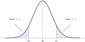
Figure 1. showing a 2-tail test for non-directional hypothesis for z for area C is the critical rejection region.
When a research hypothesis predicts a direction for the effect, it is called a directional hypothesis . To test the significance of a directional hypothesis, we have to consider the possibility that the sample could be extreme at one-tail of the comparison distribution. We call this a one-tailed test .
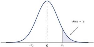
Figure 2. showing a 1-tail test for a directional hypothesis (predicting an increase) for z for area C is the critical rejection region.
Determining Cutoff Scores with Two-Tailed Tests
Typically we specify an α level before analyzing the data. If the data analysis results in a probability value below the α level, then the null hypothesis is rejected; if it is not, then the null hypothesis is not rejected. In other words, if our data produce values that meet or exceed this threshold, then we have sufficient evidence to reject the null hypothesis ; if not, we fail to reject the null (we never “accept” the null). According to this perspective, if a result is significant, then it does not matter how significant it is. Moreover, if it is not significant, then it does not matter how close to being significant it is. Therefore, if the 0.05 level is being used, then probability values of 0.049 and 0.001 are treated identically. Similarly, probability values of 0.06 and 0.34 are treated identically. Note we will discuss ways to address effect size (which is related to this challenge of NHST).
When setting the probability value, there is a special complication in a two-tailed test. We have to divide the significance percentage between the two tails. For example, with a 5% significance level, we reject the null hypothesis only if the sample is so extreme that it is in either the top 2.5% or the bottom 2.5% of the comparison distribution. This keeps the overall level of significance at a total of 5%. A one-tailed test does have such an extreme value but with a one-tailed test only one side of the distribution is considered.
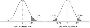
Figure 3. Critical value differences in one and two-tail tests. Photo Credit
Let’s re view th e set critical values for Z.
We discussed z-scores and probability in chapter 8. If we revisit the z-score for 5% and 1%, we can identify the critical regions for the critical rejection areas from the unit standard normal table.
- A two-tailed test at the 5% level has a critical boundary Z score of +1.96 and -1.96
- A one-tailed test at the 5% level has a critical boundary Z score of +1.64 or -1.64
- A two-tailed test at the 1% level has a critical boundary Z score of +2.58 and -2.58
- A one-tailed test at the 1% level has a critical boundary Z score of +2.33 or -2.33.
Review: Critical values, p-values, and significance level
There are two criteria we use to assess whether our data meet the thresholds established by our chosen significance level, and they both have to do with our discussions of probability and distributions. Recall that probability refers to the likelihood of an event, given some situation or set of conditions. In hypothesis testing, that situation is the assumption that the null hypothesis value is the correct value, or that there is no effec t. The value laid out in H 0 is our condition under which we interpret our results. To reject this assumption, and thereby reject the null hypothesis, we need results that would be very unlikely if the null was true.
Now recall that values of z which fall in the tails of the standard normal distribution represent unlikely values. That is, the proportion of the area under the curve as or more extreme than z is very small as we get into the tails of the distribution. Our significance level corresponds to the area under the tail that is exactly equal to α: if we use our normal criterion of α = .05, then 5% of the area under the curve becomes what we call the rejection region (also called the critical region) of the distribution. This is illustrated in Figure 4.

Figure 4: The rejection region for a one-tailed test
The shaded rejection region takes us 5% of the area under the curve. Any result which falls in that region is sufficient evidence to reject the null hypothesis.
The rejection region is bounded by a specific z-value, as is any area under the curve. In hypothesis testing, the value corresponding to a specific rejection region is called the critical value, z crit (“z-crit”) or z* (hence the other name “critical region”). Finding the critical value works exactly the same as finding the z-score corresponding to any area under the curve like we did in Unit 1. If we go to the normal table, we will find that the z-score corresponding to 5% of the area under the curve is equal to 1.645 (z = 1.64 corresponds to 0.0405 and z = 1.65 corresponds to 0.0495, so .05 is exactly in between them) if we go to the right and -1.645 if we go to the left. The direction must be determined by your alternative hypothesis, and drawing then shading the distribution is helpful for keeping directionality straight.
Suppose, however, that we want to do a non-directional test. We need to put the critical region in both tails, but we don’t want to increase the overall size of the rejection region (for reasons we will see later). To do this, we simply split it in half so that an equal proportion of the area under the curve falls in each tail’s rejection region. For α = .05, this means 2.5% of the area is in each tail, which, based on the z-table, corresponds to critical values of z* = ±1.96. This is shown in Figure 5.

Figure 5: Two-tailed rejection region
Thus, any z-score falling outside ±1.96 (greater than 1.96 in absolute value) falls in the rejection region. When we use z-scores in this way, the obtained value of z (sometimes called z-obtained) is something known as a test statistic, which is simply an inferential statistic used to test a null hypothesis.
Calculate the test statistic: Z
Now that we understand setting up the hypothesis and determining the outcome, let’s examine hypothesis testing with z! The next step is to carry out the study and get the actual results for our sample. Central to hypothesis test is comparison of the population and sample means. To make our calculation and determine where the sample is in the hypothesized distribution we calculate the Z for the sample data.
Make a decision
To decide whether to reject the null hypothesis, we compare our sample’s Z score to the Z score that marks our critical boundary. If our sample Z score falls inside the rejection region of the comparison distribution (is greater than the z-score critical boundary) we reject the null hypothesis.
The formula for our z- statistic has not changed:

To formally test our hypothesis, we compare our obtained z-statistic to our critical z-value. If z obt > z crit , that means it falls in the rejection region (to see why, draw a line for z = 2.5 on Figure 1 or Figure 2) and so we reject H 0 . If z obt < z crit , we fail to reject. Remember that as z gets larger, the corresponding area under the curve beyond z gets smaller. Thus, the proportion, or p-value, will be smaller than the area for α, and if the area is smaller, the probability gets smaller. Specifically, the probability of obtaining that result, or a more extreme result, under the condition that the null hypothesis is true gets smaller.
Conversely, if we fail to reject, we know that the proportion will be larger than α because the z-statistic will not be as far into the tail. This is illustrated for a one- tailed test in Figure 6.

Figure 6. Relation between α, z obt , and p
When the null hypothesis is rejected, the effect is said to be statistically significant . Do not confuse statistical significance with practical significance. A small effect can be highly significant if the sample size is large enough.
Why does the word “significant” in the phrase “statistically significant” mean something so different from other uses of the word? Interestingly, this is because the meaning of “significant” in everyday language has changed. It turns out that when the procedures for hypothesis testing were developed, something was “significant” if it signified something. Thus, finding that an effect is statistically significant signifies that the effect is real and not due to chance. Over the years, the meaning of “significant” changed, leading to the potential misinterpretation.
Review: Steps of the Hypothesis Testing Process
The process of testing hypotheses follows a simple four-step procedure. This process will be what we use for the remained of the textbook and course, and though the hypothesis and statistics we use will change, this process will not.
Step 1: State the Hypotheses
Your hypotheses are the first thing you need to lay out. Otherwise, there is nothing to test! You have to state the null hypothesis (which is what we test) and the alternative hypothesis (which is what we expect). These should be stated mathematically as they were presented above AND in words, explaining in normal English what each one means in terms of the research question.
Step 2: Find the Critical Values
Next, we formally lay out the criteria we will use to test our hypotheses. There are two pieces of information that inform our critical values: α, which determines how much of the area under the curve composes our rejection region, and the directionality of the test, which determines where the region will be.
Step 3: Compute the Test Statistic
Once we have our hypotheses and the standards we use to test them, we can collect data and calculate our test statistic, in this case z . This step is where the vast majority of differences in future chapters will arise: different tests used for different data are calculated in different ways, but the way we use and interpret them remains the same.
Step 4: Make the Decision
Finally, once we have our obtained test statistic, we can compare it to our critical value and decide whether we should reject or fail to reject the null hypothesis. When we do this, we must interpret the decision in relation to our research question, stating what we concluded, what we based our conclusion on, and the specific statistics we obtained.
Example: Movie Popcorn
Let’s see how hypothesis testing works in action by working through an example. Say that a movie theater owner likes to keep a very close eye on how much popcorn goes into each bag sold, so he knows that the average bag has 8 cups of popcorn and that this varies a little bit, about half a cup. That is, the known population mean is μ = 8.00 and the known population standard deviation is σ =0.50. The owner wants to make sure that the newest employee is filling bags correctly, so over the course of a week he randomly assesses 25 bags filled by the employee to test for a difference (n = 25). He doesn’t want bags overfilled or under filled, so he looks for differences in both directions. This scenario has all of the information we need to begin our hypothesis testing procedure.
Our manager is looking for a difference in the mean cups of popcorn bags compared to the population mean of 8. We will need both a null and an alternative hypothesis written both mathematically and in words. We’ll always start with the null hypothesis:
H 0 : There is no difference in the cups of popcorn bags from this employee H 0 : μ = 8.00
Notice that we phrase the hypothesis in terms of the population parameter μ, which in this case would be the true average cups of bags filled by the new employee.
Our assumption of no difference, the null hypothesis, is that this mean is exactly
the same as the known population mean value we want it to match, 8.00. Now let’s do the alternative:
H A : There is a difference in the cups of popcorn bags from this employee H A : μ ≠ 8.00
In this case, we don’t know if the bags will be too full or not full enough, so we do a two-tailed alternative hypothesis that there is a difference.
Our critical values are based on two things: the directionality of the test and the level of significance. We decided in step 1 that a two-tailed test is the appropriate directionality. We were given no information about the level of significance, so we assume that α = 0.05 is what we will use. As stated earlier in the chapter, the critical values for a two-tailed z-test at α = 0.05 are z* = ±1.96. This will be the criteria we use to test our hypothesis. We can now draw out our distribution so we can visualize the rejection region and make sure it makes sense

Figure 7: Rejection region for z* = ±1.96
Step 3: Calculate the Test Statistic
Now we come to our formal calculations. Let’s say that the manager collects data and finds that the average cups of this employee’s popcorn bags is ̅X = 7.75 cups. We can now plug this value, along with the values presented in the original problem, into our equation for z:
So our test statistic is z = -2.50, which we can draw onto our rejection region distribution:

Figure 8: Test statistic location
Looking at Figure 5, we can see that our obtained z-statistic falls in the rejection region. We can also directly compare it to our critical value: in terms of absolute value, -2.50 > -1.96, so we reject the null hypothesis. We can now write our conclusion:
When we write our conclusion, we write out the words to communicate what it actually means, but we also include the average sample size we calculated (the exact location doesn’t matter, just somewhere that flows naturally and makes sense) and the z-statistic and p-value. We don’t know the exact p-value, but we do know that because we rejected the null, it must be less than α.
Effect Size
When we reject the null hypothesis, we are stating that the difference we found was statistically significant, but we have mentioned several times that this tells us nothing about practical significance. To get an idea of the actual size of what we found, we can compute a new statistic called an effect size. Effect sizes give us an idea of how large, important, or meaningful a statistically significant effect is.
For mean differences like we calculated here, our effect size is Cohen’s d :
Effect sizes are incredibly useful and provide important information and clarification that overcomes some of the weakness of hypothesis testing. Whenever you find a significant result, you should always calculate an effect size
| d | Interpretation |
|---|---|
| 0.0 – 0.2 | negligible |
| 0.2 – 0.5 | small |
| 0.5 – 0.8 | medium |
| 0.8 – | large |
Table 1. Interpretation of Cohen’s d
Example: Office Temperature
Let’s do another example to solidify our understanding. Let’s say that the office building you work in is supposed to be kept at 74 degree Fahrenheit but is allowed
to vary by 1 degree in either direction. You suspect that, as a cost saving measure, the temperature was secretly set higher. You set up a formal way to test your hypothesis.
You start by laying out the null hypothesis:
H 0 : There is no difference in the average building temperature H 0 : μ = 74
Next you state the alternative hypothesis. You have reason to suspect a specific direction of change, so you make a one-tailed test:
H A : The average building temperature is higher than claimed H A : μ > 74

Now that you have everything set up, you spend one week collecting temperature data:
| Day | Temp |
| Monday | 77 |
| Tuesday | 76 |
| Wednesday | 74 |
| Thursday | 78 |
| Friday | 78 |
You calculate the average of these scores to be 𝑋̅ = 76.6 degrees. You use this to calculate the test statistic, using μ = 74 (the supposed average temperature), σ = 1.00 (how much the temperature should vary), and n = 5 (how many data points you collected):
z = 76.60 − 74.00 = 2.60 = 5.78
1.00/√5 0.45
This value falls so far into the tail that it cannot even be plotted on the distribution!

Figure 7: Obtained z-statistic
You compare your obtained z-statistic, z = 5.77, to the critical value, z* = 1.645, and find that z > z*. Therefore you reject the null hypothesis, concluding: Based on 5 observations, the average temperature (𝑋̅ = 76.6 degrees) is statistically significantly higher than it is supposed to be, z = 5.77, p < .05.
d = (76.60-74.00)/ 1= 2.60
The effect size you calculate is definitely large, meaning someone has some explaining to do!
Example: Different Significance Level
First, let’s take a look at an example phrased in generic terms, rather than in the context of a specific research question, to see the individual pieces one more time. This time, however, we will use a stricter significance level, α = 0.01, to test the hypothesis.
We will use 60 as an arbitrary null hypothesis value: H 0 : The average score does not differ from the population H 0 : μ = 50
We will assume a two-tailed test: H A : The average score does differ H A : μ ≠ 50
We have seen the critical values for z-tests at α = 0.05 levels of significance several times. To find the values for α = 0.01, we will go to the standard normal table and find the z-score cutting of 0.005 (0.01 divided by 2 for a two-tailed test) of the area in the tail, which is z crit * = ±2.575. Notice that this cutoff is much higher than it was for α = 0.05. This is because we need much less of the area in the tail, so we need to go very far out to find the cutoff. As a result, this will require a much larger effect or much larger sample size in order to reject the null hypothesis.
We can now calculate our test statistic. The average of 10 scores is M = 60.40 with a µ = 60. We will use σ = 10 as our known population standard deviation. From this information, we calculate our z-statistic as:
Our obtained z-statistic, z = 0.13, is very small. It is much less than our critical value of 2.575. Thus, this time, we fail to reject the null hypothesis. Our conclusion would look something like:
Notice two things about the end of the conclusion. First, we wrote that p is greater than instead of p is less than, like we did in the previous two examples. This is because we failed to reject the null hypothesis. We don’t know exactly what the p- value is, but we know it must be larger than the α level we used to test our hypothesis. Second, we used 0.01 instead of the usual 0.05, because this time we tested at a different level. The number you compare to the p-value should always be the significance level you test at. Because we did not detect a statistically significant effect, we do not need to calculate an effect size. Note: some statisticians will suggest to always calculate effects size as a possibility of Type II error. Although insignificant, calculating d = (60.4-60)/10 = .04 which suggests no effect (and not a possibility of Type II error).
Review Considerations in Hypothesis Testing
Errors in hypothesis testing.
Keep in mind that rejecting the null hypothesis is not an all-or-nothing decision. The Type I error rate is affected by the α level: the lower the α level the lower the Type I error rate. It might seem that α is the probability of a Type I error. However, this is not correct. Instead, α is the probability of a Type I error given that the null hypothesis is true. If the null hypothesis is false, then it is impossible to make a Type I error. The second type of error that can be made in significance testing is failing to reject a false null hypothesis. This kind of error is called a Type II error.
Statistical Power
The statistical power of a research design is the probability of rejecting the null hypothesis given the sample size and expected relationship strength. Statistical power is the complement of the probability of committing a Type II error. Clearly, researchers should be interested in the power of their research designs if they want to avoid making Type II errors. In particular, they should make sure their research design has adequate power before collecting data. A common guideline is that a power of .80 is adequate. This means that there is an 80% chance of rejecting the null hypothesis for the expected relationship strength.
Given that statistical power depends primarily on relationship strength and sample size, there are essentially two steps you can take to increase statistical power: increase the strength of the relationship or increase the sample size. Increasing the strength of the relationship can sometimes be accomplished by using a stronger manipulation or by more carefully controlling extraneous variables to reduce the amount of noise in the data (e.g., by using a within-subjects design rather than a between-subjects design). The usual strategy, however, is to increase the sample size. For any expected relationship strength, there will always be some sample large enough to achieve adequate power.
Inferential statistics uses data from a sample of individuals to reach conclusions about the whole population. The degree to which our inferences are valid depends upon how we selected the sample (sampling technique) and the characteristics (parameters) of population data. Statistical analyses assume that sample(s) and population(s) meet certain conditions called statistical assumptions.
It is easy to check assumptions when using statistical software and it is important as a researcher to check for violations; if violations of statistical assumptions are not appropriately addressed then results may be interpreted incorrectly.
Learning Objectives
Having read the chapter, students should be able to:
- Conduct a hypothesis test using a z-score statistics, locating critical region, and make a statistical decision including.
- Explain the purpose of measuring effect size and power, and be able to compute Cohen’s d.
Exercises – Ch. 10
- List the main steps for hypothesis testing with the z-statistic. When and why do you calculate an effect size?
- z = 1.99, two-tailed test at α = 0.05
- z = 1.99, two-tailed test at α = 0.01
- z = 1.99, one-tailed test at α = 0.05
- You are part of a trivia team and have tracked your team’s performance since you started playing, so you know that your scores are normally distributed with μ = 78 and σ = 12. Recently, a new person joined the team, and you think the scores have gotten better. Use hypothesis testing to see if the average score has improved based on the following 8 weeks’ worth of score data: 82, 74, 62, 68, 79, 94, 90, 81, 80.
- A study examines self-esteem and depression in teenagers. A sample of 25 teens with a low self-esteem are given the Beck Depression Inventory. The average score for the group is 20.9. For the general population, the average score is 18.3 with σ = 12. Use a two-tail test with α = 0.05 to examine whether teenagers with low self-esteem show significant differences in depression.
- You get hired as a server at a local restaurant, and the manager tells you that servers’ tips are $42 on average but vary about $12 (μ = 42, σ = 12). You decide to track your tips to see if you make a different amount, but because this is your first job as a server, you don’t know if you will make more or less in tips. After working 16 shifts, you find that your average nightly amount is $44.50 from tips. Test for a difference between this value and the population mean at the α = 0.05 level of significance.
Answers to Odd- Numbered Exercises – Ch. 10
1. List hypotheses. Determine critical region. Calculate z. Compare z to critical region. Draw Conclusion. We calculate an effect size when we find a statistically significant result to see if our result is practically meaningful or important
5. Step 1: H 0 : μ = 42 “My average tips does not differ from other servers”, H A : μ ≠ 42 “My average tips do differ from others”
Introduction to Statistics for Psychology Copyright © 2021 by Alisa Beyer is licensed under a Creative Commons Attribution-NonCommercial-ShareAlike 4.0 International License , except where otherwise noted.
Share This Book
Z Table. Z Score Table. Normal Distribution Table. Standard Normal Table.
What is Z-Test?
Z-Test is a statistical test which let’s us approximate the distribution of the test statistic under the null hypothesis using normal distribution .
Z-Test is a test statistic commonly used in hypothesis test when the sample data is large.For carrying out the Z-Test, population parameters such as mean, variance, and standard deviation should be known.
This test is widely used to determine whether the mean of the two samples are different when the variance is known. We make use of the Z score and the Z table for running the Z-Test.
Z-Test as Hypothesis Test
A test statistic is a random variable that we calculate from the sample data to determine whether to reject the null hypothesis. This random variable is used to calculate the P-value, which indicates how strong the evidence is against the null hypothesis. Z-Test is such a test statistic where we make use of the mean value and z score to determine the P-value. Z-Test compares the mean of two large samples taken from a population when the variance is known.
Z-Test is usually used to conduct a hypothesis test when the sample size is greater than 30. This is because of the central limit theorem where when the sample gets larger, the distributed data graph starts resembling a bell curve and is considered to be distributed normally. Since the Z-Test follows normal distribution under the null hypothesis, it is the most suitable test statistic for large sample data.
Why do we use a large sample for conducting a hypothesis test?
In a hypothesis test, we are trying to reject a null hypothesis with the evidence that we should collect from sample data which represents only a portion of the population. When the population has a large size, and the sample data is small, we will not be able to draw an accurate conclusion from the test to prove our null hypothesis is false. As sample data provide us a door to the entire population, it should be large enough for us to arrive at a significant inference. Hence a sufficiently large data should be considered for a hypothesis test especially if the population is huge.
How to Run a Z-Test
Z-Test can be considered as a test statistic for a hypothesis test to calculate the P-value. However, there are certain conditions that should be satisfied by the sample to run the Z-Test.
The conditions are as follows:
- The sample size should be greater than 30.
This is already mentioned above. The size of the sample is an important factor in Z-Testing as the Z-Test follows a normal distribution and so should the data. If the same size is less than 30, it is recommended to use a t-test instead
- All the data point should be independent and doesn’t affect each other.
Each element in the sample, when considered single should be independent and shouldn’t have a relationship with another element.
- The data must be distributed normally.
This is ensured if the sample data is large.
- The sample should be selected randomly from a population.
Each data in the population should have an equal chance to be selected as one of the sample data.
- The sizes of the selected samples should be equal if at all possible.
When considering multiple sample data, ensuring that the size of each sample is the same for an accurate calculation of population parameters.
- The standard deviation of the population is known.
The population parameter, standard deviation must be given to run a Z-Test as we cannot perform the calculation without knowing it. If it is not directly given, then it assumed that the variance of the sample data is equal to the variance of the entire population.
If the conditions are satisfied, the Z-Test can be successfully implemented.
Following are steps to run the Z-Test:
- State the null hypothesis
The null hypothesis is a statement of no effect and it supports the data which is already given. It is generally represented as :
- State the alternate hypothesis
The statement that we are trying to prove is the alternate hypothesis. It is represented as:
This is the representation of a bidirectional alternate hypothesis.
- H 1 :µ > k
This is the representation of a one-directional alternate hypothesis that is represented in the right region of the graph.
- H 1 :µ < k
This is the representation of a one-directional alternate hypothesis that is represented in the left region of the graph.
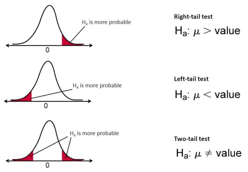
- Choose an alpha level for the test.
Alpha level or significant level is the probability of rejecting the null hypothesis when it is true. It is represented by ( α ). An alpha level must be chosen wisely so as to avoid the Type I and Type II errors.
If we choose a large alpha value such as 10%, it is likely to reject a null hypothesis when it is true. There is a probability of 10% for us to reject the null hypothesis. This is an error known as the Type I error.
On the other hand, if we choose an alpha level as low as 1%, there is a chance to accept the null hypothesis even if it is false. That is we reject the alternate hypothesis to favor the null hypothesis. This is the Type II error.
Hence the alpha level should be chosen in such a way that the chance of making Type I or Type II error is minimal. For this reason, the alpha level is commonly selected as 5% which is proven best to avoid errors.
- Determining the critical value of Z from the Z table.
The critical value is the point in the normal distribution graph that splits the graph into two regions: the acceptance region and the rejection regions. It can be also described as the extreme value for which a null hypothesis can be accepted. This critical value of Z can be found from the Z table .
- Calculate the test statistic.
The sample data that we choose to test is converted into a single value. This is known as the test statistic. This value is compared to the null value. If the test statistic significantly differs from the null value, the null value is rejected.
- Comparing the test statistic with the critical value.
Now, we have to determine whether the test statistic we have calculated comes under the acceptance region or the rejection region. For this, the test statistic is compared with the critical value to know whether we should accept or reject a null hypothesis.
Types of Z-Test
Z-Test can be used to run a hypothesis test for a single sample or to compare the mean of two samples. There are two common types of Z-Test
One-Sample Z-Test
This is the most basic type of hypothesis test that is widely used. For running an one-sample Z-Test, all we need to know is the mean and standard deviation of the population. We consider only a single sample for a one-sample Z-Test. One-sample Z-Test is used to test whether the population parameter is different from the hypothesized value i.e whether the mean of the population is equal to, less than or greater than the hypothesized value.
The equation for finding the value of Z is:
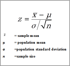
The following are the assumptions that are generally taken for a one-sampled Z-Test:
- The sample size is equal to or greater than 30.
- One normally distributed sample is considered with the standard deviation known.
- The null hypothesis is that the population mean that is calculated from the sample is equal to the hypothetically determined population mean.
Two-Sample Z-Test
A two-sample Z-Test is used whenever there is a comparison between two independent samples. It is used to check whether the difference between the means is equal to zero or not. Suppose if we want to know whether men or women prefer to drive more in a city, we use a two-sample Z-Test as it is the comparison of two independent samples of men and women.
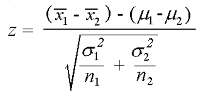
- x 1 and x 2 represent the mean of the two samples.
- µ 1 and µ 2 are the hypothesized mean values.
- σ 1 and σ 2 are the standard deviations.
- n 1 and n 2 are the sizes of the samples.
The following are the assumptions that are generally taken for a two-sample Z-Test:
- Two independent, normally distributed samples are considered for the Z-Test with the standard deviation known.
- Each sample is equal to or greater than 30.
- The null hypothesis is stated that the population mean of the two samples taken does not differ.
Critical value
A critical value is a line that splits a normally distributed graph into two different sections. Namely the ‘Rejection region’ and ‘Acceptance region’. If your test value falls in the ‘Rejection region’, then the null hypothesis is rejected and if your test value falls in the ‘Accepted region’, then the null hypothesis is accepted.
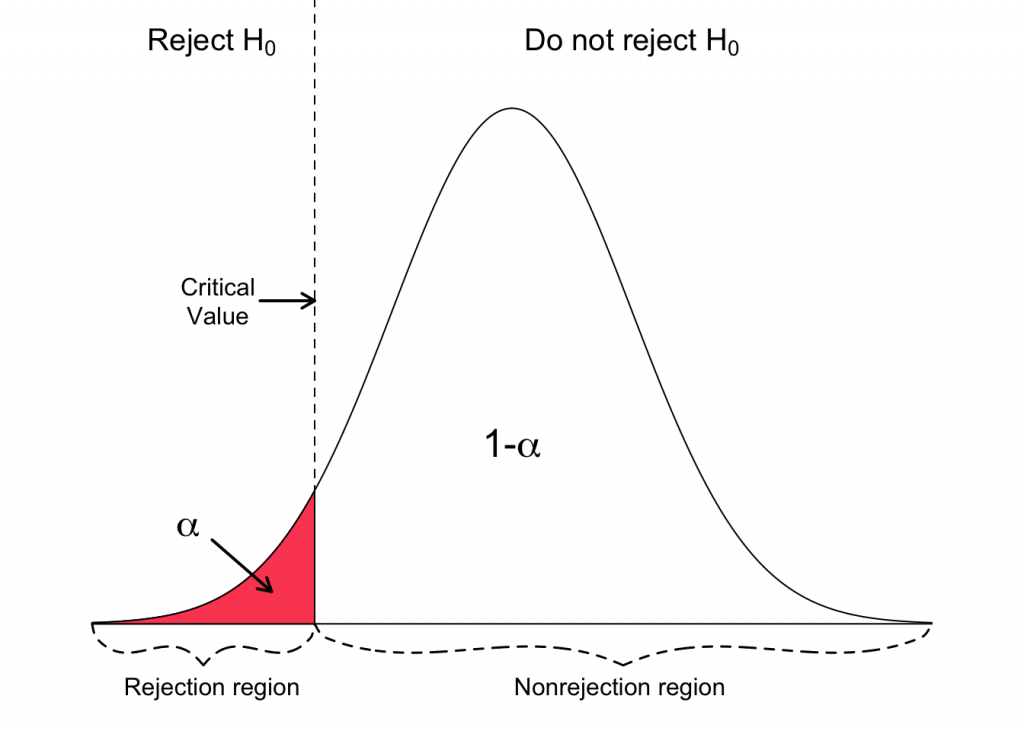
Critical Value Vs Significant Value
Significant level, alpha is the probability of rejecting a null hypothesis when it is actually true. While the critical value is the extreme value up to which a null hypothesis is true. There migh come a confusion regarding both of these parameters.
Critical value is a value that lies in critical region. It is in fact the boundary value of the rejection region. Also, it is the value up to which the null hypothesis is true. Hence the critical value is considered to be the point at which the null hypothesis is true or is rejected.
Critical value gives a point of extremity whose probability is indicated by the significant level. Significant level is pre-selected for a hypothesis test and critical value is calculated from this Alpha value. Critical value is a point represented as Z score and Significant level is a probability.
Z-Test Vs T-Test
Z-Test are used when the sample size exceeds 30. As Z-Test follows normal distribution, large sample size can be taken for the Z-Test. Z-Test indicates the distance of a data point from the mean of the data set in terms of standard deviation. Also. this test can only be used if the standard deviation of the data set is known.
T-Test is based on T distribution in which the mean value is known and the variance could be calculated from the sample. T-Test is most preferred to know the difference between the statistical parameters of two samples as the standard deviation of the samples are not usually given in a two-sample test for running the Z-Test. Also, if the sample size is less than 30, T-Test is preferred.
Approximate Hypothesis Tests: the z Test and the t Test
This chapter presents two common tests of the hypothesis that a population mean equals a particular value and of the hypothesis that two population means are equal: the z test and the t test. These tests are approximate : They are based on approximations to the probability distribution of the test statistic when the null hypothesis is true, so their significance levels are not exactly what they claim to be. If the sample size is reasonably large and the population from which the sample is drawn has a nearly normal distribution —a notion defined in this chapter—the nominal significance levels of the tests are close to their actual significance levels. If these conditions are not met, the significance levels of the approximate tests can differ substantially from their nominal values. The z test is based on the normal approximation ; the t test is based on Student's t curve, which approximates some probability histograms better than the normal curve does. The chapter also presents the deep connection between hypothesis tests and confidence intervals, and shows how to compute approximate confidence intervals for the population mean of nearly normal populations using Student's t -curve.
where \(\phi\) is the pooled sample percentage of the two samples. The estimate of \(SE(\phi^{t-c})\) under the null hypothesis is
\[ se = s^*\times(1/n_t + 1/n_c)^{1/2}, \]
where \(n_t\) and \(n_c\) are the sizes of the two samples. If the null hypothesis is true, the Z statistic,
\[ Z=\phi^{t-c}/se, \]
is the original test statistic \(\phi^{t-c}\) in approximately standard units , and Z has a probability histogram that is approximated well by the normal curve , which allowed us to select the rejection region for the approximate test.
This strategy—transforming a test statistic approximately to standard units under the assumption that the null hypothesisis true, and then using the normal approximation to determine the rejection region for the test—works to construct approximate hypothesis tests in many other situations, too. The resulting hypothesis test is called a z test. Suppose that we are testing a null hypothesis using a test statistic \(X\) , and the following conditions hold:
- We have a probability model for how the observations arise, assuming the null hypothesis is true. Typically, the model is that under the null hypothesis, the data are like random draws with or without replacement from a box of numbered tickets.
- Under the null hypothesis, the test statistic \(X\) , converted to standard units, has a probability histogram that can be approximated well by the normal curve.
- Under the null hypothesis, we can find the expected value of the test statistic, \(E(X)\) .
- Under the null hypothesis, either we can find the SE of the test statistic, \(SE(X)\) , or we can estimate \(SE(X)\) accurately enough to ignore the error of the estimate of the SE. Let se denote either the exact SE of \(X\) under the null hypothesis, or the estimated value of \(SE(X)\) under the null hypothesis.
Then, under the null hypothesis, the probability histogram of the Z statistic
\[ Z = (X-E(X))/se \]
is approximated well by the normal curve, and we can use the normal approximation to select the rejection region for the test using \(Z\) as the test statistic. If the null hypothesis is true,
\[ P(Z < z_a) \approx a \]
\[ P(Z > z_{1-a} ) \approx a, \]
\[ P(|Z| > z_{1-a/2} ) \approx a. \]
These three approximations yield three different z tests of the hypothesis that \(\mu = \mu_0\) at approximate significance level \(a\) :
- Reject the null hypothesis whenever \(Z (left-tail z test)
- Reject the null hypothesis whenever \(Z > z_{1-a}\) (right-tail z test)
- Reject the null hypothesis whenever \(|Z|> z_{1-a/2}\) (two-tail z test)
The word "tail" refers to the tails of the normal curve: In a left-tail test, the probability of a Type I error is approximately the area of the left tail of the normal curve, from minus infinity to \(z_a\) . In a right-tail test, the probability of a Type I error is approximately the area of the right tail of the normal curve, from \(z_{1-a}\) to infinity. In a two-tail test, the probability of a Type I error is approximately the sum of the areas of both tails of the normal curve, the left tail from minus infinity to \(z_{a/2}\) and the right tail from \(z_{1-a/2}\) to infinity. All three of these tests are called z tests. The observed value of Z is called the z score .
Which of these three tests, if any, should one use? The answer depends on the probability distribution of Z when the alternative hypothesis is true. As a rule of thumb, if, under the alternative hypothesis, \(E(Z) , use the left-tail test. If, under the alternative hypothesis, \(E(Z) > 0\) , use the right-tail test. If, under the alternative hypothesis, it is possible that \(E(Z) and it is possible that \(E(Z) > 0\) , use the two-tail test. If, under the alternative hypothesis, \(E(Z) = 0\) , consult a statistician. Generally (but not always), this rule of thumb selects the test with the most power for a given significance level.
P values for z tests
Each of the three z tests gives us a family of procedures for testing the null hypothesis at any (approximate) significance level \(a\) between 0 and 100%—we just use the appropriate quantile of the normal curve. This makes it particularly easy to find the P value for a z test. Recall that the P value is the smallest significance level for which we would reject the null hypothesis, among a family of tests of the null hypothesis at different significance levels.
Suppose the z score (the observed value of \(Z\) ) is \(x\) . In a left-tail test, the P value is the area under the normal curve to the left of \(x\) : Had we chosen the significance level \(a\) so that \(z_a=x\) , we would have rejected the null hypothesis, but we would not have rejected it for any smaller value of \(a\) , because for all smaller values of \(a\) , \(z_a . Similarly, for a right-tail z test, the P value is the area under the normal curve to the right of \(x\) : If \(x=z_{1-a}\) we would reject the null hypothesis at approximate significance level \(a\) , but not at smaller significance levels. For a two-tail z test, the P value is the sum of the area under the normal curve to the left of \(-|x|\) and the area under the normal curve to the right of \(|x|\) .
Finding P values and specifying the rejection region for the z test involves the probability distribution of \(Z\) under the assumption that the null hypothesis is true. Rarely is the alternative hypothesis sufficiently detailed to specify the probability distribution of \(Z\) completely, but often the alternative does help us choose intelligently among left-tail, right-tail, and two-tail z tests. This is perhaps the most important issue in deciding which hypothesis to take as the null hypothesis and which as the alternative: We calculate the significance level under the null hypothesis, and that calculation must be tractable.
However, to construct a z test, we need to know the expected value and SE of the test statistic under the null hypothesis. Usually it is easy to determine the expected value, but often the SE must be estimated from the data. Later in this chapter we shall see what to do if the SE cannot be estimated accurately, but the shape of the distribution of the numbers in the population is known. The next section develops z tests for the population percentage and mean, and for the difference between two population means.
Examples of z tests
The central limit theorem assures us that the probability histogram of the sample mean of random draws with replacement from a box of tickets—transformed to standard units—can be approximated increasingly well by a normal curve as the number of draws increases. In the previous section, we learned that the probability histogram of a sum or difference of independent sample means of draws with replacement also can be approximated increasingly well by a normal curve as the two sample sizes increase. We shall use these facts to derive z tests for population means and percentages and differences of population means and percentages.
z Test for a Population Percentage
Suppose we have a population of \(N\) units of which \(G\) are labeled "1" and the rest are labeled "0." Let \(p = G/N\) be the population percentage. Consider testing the null hypothesis that \(p = p_0\) against the alternative hypothesis that \(p \ne p_0\) , using a random sample of \(n\) units drawn with replacement. (We could assume instead that \(N >> n\) and allow the draws to be without replacement.)
Under the null hypothesis, the sample percentage
\[ \phi = \frac{\mbox{# tickets labeled "1" in the sample}}{n} \]
has expected value \(E(\phi) = p_0\) and standard error
\[ SE(\phi) = \sqrt{\frac{p_0 \times (1 - p_0)}{n}}. \]
Let \(Z\) be \(\phi\) transformed to standard units :
\[ Z = (\phi - p_0)/SE(\phi). \]
Provided \(n\) is large and \(p_0\) is not too close to zero or 100% (say \(n \times p > 30\) and \(n \times (1-p) > 30)\) , the probability histogram of \(Z\) will be approximated reasonably well by the normal curve, and we can use it as the Z statistic in a z test. For example, if we reject the null hypothesis when \(|Z| > 1.96\) , the significance level of the test will be about 95%.
z Test for a Population Mean
The approach in the previous subsection applies, mutatis mutandis , to testing the hypothesis that the population mean equals a given value, even when the population contains numbers other than just 0 and 1. However, in contrast to the hypothesis that the population percentage equals a given value, the null hypothesis that a more general population mean equals a given value does not specify the SD of the population, which poses difficulties that are surmountable (by approximation and estimation) if the sample size is large enough. (There are also nonparametric methods that can be used.)
Consider testing the null hypothesis that the population mean \(\mu\) is equal to a specific null value \(\mu_0\) , against the alternative hypothesis that \(\mu , on the basis of a random sample with replacement of size \(n\) . Recall that the sample mean \(M\) of \(n\) random draws with or without replacement from a box of numbered tickets is an unbiased estimator of the population mean \(\mu\) : If
\[ M = \frac{\mbox{sum of sample values}}{n}, \]
\[ E(M) = \mu = \frac{\mbox{sum of population values}}{N}, \]
where \(N\) is the size of the population. The population mean determines the expected value of the sample mean. The SE of the sample mean of a random sample with replacement is
\[ \frac{SD(\mbox{box})}{\sqrt{n}}, \]
where SD(box) is the SD of the list of all the numbers in the box, and \(n\) is the sample size. As a special case, the sample percentage \phi of \(n\) independent random draws from a 0-1 box is an unbiased estimator of the population percentage p , with SE equal to
\[ \sqrt{\frac{p\times(1-p)}{n}}. \]
In testing the null hypothesis that a population percentage \(p\) equals \(p_0\) , the null hypothesis specifies not only the expected value of the sample percentage \phi, it automatically specifies the SE of the sample percentage as well, because the SD of the values in a 0-1 box is determined by the population percentage \(p\) :
\[ SD(box) = \sqrt{p\times(1-p)}. \]
The null hypothesis thus gives us all the information we need to standardize the sample percentage under the null hypothesis. In contrast, the SD of the values in a box of tickets labeled with arbitrary numbers bears no particular relation to the mean of the values, so the null hypothesis that the population mean \(\mu\) of a box of tickets labeled with arbitrary numbers equals a specific value \(\mu_0\) determines the expected value of the sample mean, but not the standard error of the sample mean. To standardize the sample mean to construct a z test for the value of a population mean, we need to estimate the SE of the sample mean under the null hypothesis. When the sample size is large, the sample standard deviation s> is likely to be close to the SD of the population, and
\[ se=\frac{s}{\sqrt{n}} \]
is likely to be an accurate estimate of \(SE(M)\) . The central limit theorem tells us that when the sample size \(n\) is large, the probability histogram of the sample mean, converted to standard units, is approximated well by the normal curve. Under the null hypothesis,
\[ E(M) = \mu_0, \]
and thus when \(n\) is large
\[ Z = \frac{M-\mu_0}{s/\sqrt{n}} \]
has expected value zero, and its probability histogram is approximated well by the normal curve, so we can use \(Z\) as the Z statistic in a z test. If the alternative hypothesis is true, the expected value of \(Z\) could be either greater than zero or less than zero, so it is appropriate to use a two-tail z test. If the alternative hypothesis is \(\mu > \mu_0\) , then under the alternative hypothesis, the expected value of \(Z\) is greater than zero, and it is appropriate to use a right-tail z test. If the alternative hypothesis is \(\mu , then under the alternative hypothesis, the expected value of \(Z\) is less than zero, and it is appropriate to use a left-tail z test.
z Test for a Difference of Population Means
Consider the problem of testing the hypothesis that two population means are equal, using random samples from the two populations. Different sampling designs lead to different hypothesis testing procedures. In this section, we consider two kinds of random samples from the two populations: paired samples and independent samples , and construct z tests appropriate for each.
Paired Samples
Consider a population of \(N\) individuals, each of whom is labeled with two numbers. For example, the \(N\) individuals might be a group of doctors, and the two numbers that label each doctor might be the annual payments to the doctor by an HMO under the terms of the current contract and under the terms of a proposed revision of the contract. Let the two numbers associated with individual \(i\) be \(c_i\) and \(t_i\) . (Think of \(c\) as control and \(t\) as treatment . In this example, control is the current contract, and treatment is the proposed contract.) Let \(\mu_c\) be the population mean of the \(N\) values
\[ \{c_1, c_2, \ldots, c_N \}, \]
and let \(\mu_t\) be the population mean of the \(N\) values
\[ \{t_1, t_2, \ldots, t_N\}. \]
Suppose we want to test the null hypothesis that
\[ \mu = \mu_t - \mu_c = \mu_0 \]
against the alternative hypothesis that \(\mu . With \(\mu_0=\$0\) , this null hypothesis is that the average annual payment to doctors under the proposed revision would be the same as the average payment under the current contract, and the alternative is that on average doctors would be paid less under the new contract than under the current contract. With \(\mu_0=-\$5,000\) , this null hypothesis is that the proposed contract would save the HMO an average of $5,000 per doctor, compared with the current contract; the alternative is that under the proposed contract, the HMO would save even more than that. With \(\mu_0=\$1,000\) , this null hypothesis is that doctors would be paid an average of $1,000 more per year under the new contract than under the old one; the alternative hypothesis is that on average doctors would be paid less than an additional $1,000 per year under the new contract—perhaps even less than they are paid under the current contract. For the remainder of this example, we shall take \(\mu_0=\$1,000\) .
The data on which we shall base the test are observations of both \(c_i\) and \(t_i\) for a sample of \(n\) individuals chosen at random with replacement from the population of \(N\) individuals (or a simple random sample of size \(n ): We select \(n\) doctors at random from the \(N\) doctors under contract to the HMO, record the current annual payments to them, and calculate what the payments to them would be under the terms of the new contract. This is called a paired sample , because the samples from the population of control values and from the population of treatment values come in pairs: one value for control and one for treatment for each individual in the sample. Testing the hypothesis that the difference between two population means is equal to \(\mu_0\) using a paired sample is just the problem of testing the hypothesis that the population mean \(\mu\) of the set of differences
\[ d_i = t_i - c_i, \;\; i= 1, 2, \ldots, N, \]
is equal to \(\mu_0\) . Denote the \(n\) (random) observed values of \(c_i\) and \(t_i\) by \(\{C_1, C_2, \ldots, C_n\}\) and \(\{T_1, T_2, \ldots, T_n \}\) , respectively. The sample mean \(M\) of the differences between the observed values of \(t_i\) and \(c_i\) is the difference of the two sample means:
\[ M = \frac{(T_1-C_1)+(T_2-C_2) + \cdots + (T_n-C_n)}{n} = \frac{T_1+T_2+ \cdots + T_n}{n} - \frac{C_1+C_2+ \cdots + C_n}{n} \]
\[ = (\mbox{sample mean of observed values of } t_i) - (\mbox{sample mean of observed values of } c_i). \]
\(M\) is an unbiased estimator of \(\mu\) , and if n is large, the normal approximation to its probability histogram will be accurate. The SE of \(M\) is the population standard deviation of the \(N\) values \(\{d_1, d_2, \ldots, d_N\}\) , which we shall denote \(SD_d\) , divided by the square root of the sample size, \(n^{1/2}\) . Let \(sd\) denote the sample standard deviation of the \(n\) observed differences \((T_i - C_i), \;\; i=1, 2, \ldots, n\) :
\[ sd = \sqrt{\frac{(T_1-C_1-M)^2 + (T_2-C_2-M)^2 + \cdots + (T_n-C_n-M)^2}{n-1}} \]
(recall that \(M\) is the sample mean of the observed differences). If the sample size \(n\) is large, sd is very likely to be close to SD( d ), and so, under the null hypothesis,
\[ Z = \frac{M-\mu_0}{sd/n^{1/2}} \]
has expected value zero, and when \(n\) is large the probability histogram of \(Z\) can be approximated well by the normal curve. Thus we can use \(Z\) as the Z statistic in a z test of the null hypothesis that \(\mu=\mu_0\) . Under the alternative hypothesis that \(\mu (doctors on the average are paid less than an additional $1,000 per year under the new contract), the expected value of \(Z\) is less than zero, so we should use a left-tail z test. Under the alternative hypothesis \(\mu\ne\mu_0\) (on average, the difference in average annual payments to doctors is not an increase of $1,000, but some other number instead), the expected value of \(Z\) could be positive or negative, so we would use a two-tail z test. Under the alternative hypothesis that \(\mu>\mu_0\) (on average, under the new contract, doctors are paid more than an additional $1,000 per year), the expected value of \(Z\) would be greater than zero, so we should use a right-tail z test.
Independent Samples
Consider two separate populations of numbers, with population means \(\mu_t\) and \(\mu_c\) , respectively. Let \(\mu=\mu_t-\mu_c\) be the difference between the two population means. We would like to test the null hypothesis that \(\mu=\mu_0\) against the alternative hypothesis that \(\mu>0\) . For example, let \(\mu_t\) be the average annual payment by an HMO to doctors in the Los Angeles area, and let \(\mu_c\) be the average annual payment by the same HMO to doctors in the San Francisco area. Then the null hypothesis with \(\mu_0=0\) is that the HMO pays doctors in the two regions the same amount annually, on average; the alternative hypothesis is that the average annual payment by the HMO to doctors differs between the two areas. Suppose we draw a random sample of size \(n_t\) with replacement from the first population, and independently draw a random sample of size \(n_c\) with replacement from the second population. Let \(M_t\) and \(M_c\) be the sample means of the two samples, respectively, and let
\[ M = M_t - M_c \]
be the difference between the two sample means. Because the expected value of \(M_t\) is \(\mu_t\) and the expected value of \(M_c\) is \(\mu_c\) , the expected value of \(M\) is
\[ E(M) = E(M_t - M_c) = E(M_t) - E(M_c) = \mu_t - \mu_c = \mu. \]
Because the two random samples are independent , \(M_t\) and \(-M_c\) are independent random variables, and the SE of their sum is
\[ SE(M) = (SE^2(M_t) + SE^2(M_c))^{1/2}. \]
Let \(s_t\) and \(s_c\) be the sample standard deviations of the two samples, respectively. If \(n_t\) and \(n_c\) are both very large, the two sample standard deviations are likely to be close to the standard deviations of the corresponding populations, and so \(s_t/n_t^{1/2}\) is likely to be close to \(SE(M_t)\) , and \(s_c/n_c^{1/2}\) is likely to be close to \(SE(M_c)\) . Therefore, the pooled estimate of the standard error
\[ se_\mbox{diff} = ( (s_t/n_t^{1/2})^2 + (s_c/n_c^{1/2})^2)^{1/2} = \sqrt{ s_t^2/n_t + s_c^2/n_c} \]
is likely to be close to \(SE(M)\) . Under the null hypothesis, the statistic
\[ Z = \frac{M - \mu_0}{se_\mbox{diff}} = \frac{M_1 - M_2 - \mu_0}{\sqrt{ s_t^2/n_t + s_c^2/n_c}} \]
has expected value zero and its probability histogram is approximated well by the normal curve, so we can use it as the Z statistic in a z test.
Under the alternative hypothesis
\[ \mu = \mu_t - \mu_c > \mu_0, \]
the expected value of \(Z\) is greater than zero, so it is appropriate to use a right-tail z test.
If the alternative hypothesis were \(\mu \ne \mu_0\) , under the alternative the expected value of \(Z\) could be greater than zero or less than zero, so it would be appropriate to use a two-tail z test. If the alternative hypothesis were \(\mu , under the alternative the expected value of \(Z\) would be less than zero, so it would be appropriate to use a left-tail z test.
The following exercises check that you can compute the z test for a population mean or a difference of population means. The exercises are dynamic: the data will tend to change when you reload the page.
For the nominal significance level of the z test for a population mean to be approximately correct, the sample size typically must be large. When the sample size is small, two factors limit the accuracy of the z test: the normal approximation to the probability distribution of the sample mean can be poor, and the sample standard deviation can be an inaccurate estimate of the population standard deviation, so se is not an accurate estimate of the SE of the test statistic Z . For nearly normal populations , defined in the next subsection, the probability distribution of the sample mean is nearly normal even when the sample size is small, and the uncertainty of the sample standard deviation as an estimate of the population standard deviation can be accounted for by using a curve that is broader than the normal curve to approximate the probability distribution of the (approximately) standardized test statistic. The broader curve is Student's t curve . Student's t curve depends on the sample size: The smaller the sample size, the more spread out the curve.
Nearly Normally Distributed Populations
A list of numbers is nearly normally distributed if the fraction of values in any range is close to the area under the normal curve for the corresponding range of standard units—that is, if the list has mean \(\mu\) and standard deviation SD, and for every pair of values \(a < b\) ,
\[ \mbox{ the fraction of numbers in the list between } a \mbox{ and } b \approx \mbox{the area under the normal curve between } (a - \mu)/SD \mbox{ and } (b - \mu)/SD. \]
A list is nearly normally distributed if the normal curve is a good approximation to the histogram of the list transformed to standard units. The histogram of a list that is approximately normally distributed is (nearly) symmetric about some point, and is (nearly) bell-shaped.
No finite population can be exactly normally distributed, because the area under the normal curve between every two distinct values is strictly positive—no matter how large or small the values nor how close together they are. No population that contains only a finite number of distinct values can be exactly normally distributed, for the same reason. In particular, populations that contain only zeros and ones are not approximately normally distributed, so results for the sample mean of samples drawn from nearly normally distributed populations need not apply to the sample percentage of samples drawn from 0-1 boxes. Such results will be more accurate for the sample percentage when the population percentage is close to 50% than when the population percentage is close to 0% or 100%, because then the histogram of population values is more nearly symmetric.
Suppose a population is nearly normally distributed. Then a histogram of the population is approximately symmetric about the mean of the population. The fraction of numbers in the population within ±1 SD of the mean of the population is about 68%, the fraction of numbers within ±2 SD of the mean of the population is about 95%, and the fraction of numbers in the population within ±3 SD of the mean of the population is about 99.7%.
The following exercises check that you understand what it means for a list to be nearly normally distributed. The exercises are dynamic: the data tend to change when you reload the page.
Student's t -curve
Student's t curve is similar to the normal curve, but broader. It is positive, has a single maximum, and is symmetric about zero. The total area under Student's t curve is 100%. Student's t curve approximates some probability histograms more accurately than the normal curve does. There are actually infinitely many Student t curves, one for each positive integer value of the degrees of freedom. As the degrees of freedom increases, the difference between Student's t curve and the normal curve decreases.
Consider a population of \(N\) units labeled with numbers. Let \(\mu\) denote the population mean of the \(N\) numbers, and let SD denote the population standard deviation of the \(N\) numbers. Let \(M\) denote the sample mean of a random sample of size \(n\) drawn with replacement from a population, and let s> denote the sample standard deviation of the sample. The expected value of \(M\) is \(\mu\) , and the SE of \(M\) is \(SD/n^{1/2}\) . Let
\[ Z = (M - \mu)/(SD/n^{1/2}). \]
Then the expected value of \(Z\) is zero, the SE of \(Z\) is 1, and if \(n\) is large enough, the normal curve is a good approximation to the probability histogram of \(Z\) . The closer to normal the distribution of values in the population is, the smaller \(n\) needs to be for the normal curve to be a good approximation to the distribution of \(Z\) . Consider the statistic
\[ T = \frac{M - \mu}{s/n^{1/2}}, \]
which replaces SD by its estimated value (the sample standard deviation \(s\) ). If \(n\) is large enough, \(s\) is very likely to be close to SD, so \(T\) will be close to \(Z\) ; the normal curve will be a good approximation to the probability histogram of \(T\) ; and we can use \(T\) as the Z statistic in a z test of hypotheses about \(\mu\) .
For many populations, when the sample size is small—say less than 25, but the accuracy depends on the population—the normal curve is not a good approximation to the probability histogram of \(T\) . For nearly normally distributed populations, when the sample size is intermediate—say 25–100, but again this depends on the population—the normal curve is a good approximation to the probability histogram of \(Z\) , but not to the probability histogram of \(T\) , because of the variability of the sample standard deviation s> from sample to sample, which tends to broaden the probability distribution of \(T\) (i.e., to make \(SE(T)>1\) ).
When you first load this page, the degrees of freedom will be set to 25, and the region from -1.96 to 1.96 will be hilighted. The area under the normal curve between ±1.96 is 95%, but for Student's t curve with 25 degrees of freedom, the area is about 93.9%: Student's t curve with d.f.=25 is broader than the normal curve. Increase the degrees of freedom to 200; you will see that the Student t curve gets slightly narrower, and the area under the curve between ±1.96 is about 94.9%.
We define quantiles of Student t curves in the same way we defined quantiles of the normal curve: For any number a between 0 and 100%, the a quantile of Student's t curve with \(d.f.=d\) , \(t_{d,a}\) , is the unique value such that the area under the Student t curve with d degrees of freedom from minus infinity to \(t_{d,a}\) is equal to \(a\) . For example, \(t_{d,0.5} = 0\) for all values of \(d\) . Generally, the value of \(t_{d,a}\) depends on the degrees of freedom \(d\) . The probability calculator allows you to find quantiles of Student's t curve.
t test for the Mean of a Nearly Normally Distributed Population
We can use Student's t curve to construct approximate tests of hypotheses about the population mean \(\mu\) when the population standard deviation is unknown, for intermediate values of the sample size \(n\) . The approach is directly analogous to the z test, but instead of using a quantile of the normal curve, we use the corresponding quantile of Student's t curve (with the appropriate number of degrees of freedom). However, for the test to be accurate when \(n\) is small or intermediate, the distribution of values in the population must be nearly normal for the test to have approximately its nominal level. This is a somewhat bizarre restriction: It may require a very large sample to detect that the population is not nearly normal—but if the sample is very large, we can use the z test instead of the t test, so we don't need to rely as much on the assumption. It is my opinion that the t test is over-taught and overused—because its assumptions are not verifiable in the situations where it is potentially useful.
Consider testing the null hypothesis that \(\mu=\mu_0\) using the sample mean \(M\) and sample standard deviation s> of a random sample of size \(n\) drawn with replacement from a population that is known to have a nearly normal distribution. Define
\[ T = \frac{M - \mu_0}{s/n^{1/2}}. \]
Under the null hypothesis, if \(n\) is not too small, Student's t curve with \(n-1\) degrees of freedom will be an accurate approximation to the probability histogram of \(T\) , so
\[ P(T < t_{n-1,a}), \]
\[ P(T > t_{n-1,1-a}), \]
\[ P(|T| > t_{n-1,1-a/2}) \]
all are approximately equal to \(a\) . As we saw earlier in this chapter for the Z statistic, these three approximations give three tests of the null hypothesis \(\mu=\mu_0\) at approximate significance level \(a\) —a left-tail t test, a right-tail t test, and a two-tail t test:
- Reject the null hypothesis if \(T (left-tail)
- Reject the null hypothesis if \(T > t_{n-1,1-a}\) (right-tail)
- Reject the null hypothesis if \(|T| > t_{n-1,1-a/2}\) (two-tail)
To decide which t test to use, we can apply the same rule of thumb we used for the z test:
- Use a left-tail t test if, under the alternative hypothesis, the expected value of \(T\) is less than zero.
- Use a right-tail t test if, under the alternative hypothesis, the expected value of \(T\) is greater than zero.
- Use a two-tail t test if, under the alternative hypothesis, the expected value of \(T\) is not zero, but could be less than or greater than zero.
- Consult a statistician for a more appropriate test if, under the alternative hypothesis, the expected value of \(T\) is zero.
P-values for t tests are computed in much the same way as P-values for z tests. Let t be the observed value of \(T\) (the t score). In a left-tail t test, the P-value is the area under Student's t curve with \(n-1\) degrees of freedom, from minus infinity to \(t\) . In a right-tail t test, the P-value is the area under Student's t curve with \(n-1\) degrees of freedom, from \(t\) to infinity. In a two-tail t test, the P-value is the total area under Student's t curve with \(n-1\) degrees of freedom between minus infinity and \(-|t|\) and between \(|t|\) and infinity.
There are versions of the t test for comparing two means, as well. Just like for the z test, the method depends on how the samples from the two populations are drawn. For example, if the two samples are paired (if we are sampling individuals labeled with two numbers and for each individual in the sample, we observe both numbers), we may base the t test on the sample mean of the paired differences and the sample standard deviation of the paired differences. Let \(\mu_1\) and \(\mu_2\) be the means of the two populations, and let
\[ \mu = \mu_1 - \mu_2. \]
The \(T\) statistic to test the null hypothesis that \(\mu=\mu_0\) is
\[ T = \frac{(\mbox{sample mean of differences}) - \mu_0 }{(\mbox{sample standard deviation of differences})/n^{1/2}}, \]
and the appropriate curve to use to find the rejection region for the test is Student's t curve with \(n-1\) degrees of freedom, where \(n\) is the number of individuals (differences) in the sample.
Two-sample t tests for a difference of means using independent samples depend on additional assumptions, such as equality of the two population standard deviations; we shall not present such tests here. The following exercises check your ability to compute t tests. The exercises are dynamic: the data tend to change when you reload the page.
Hypothesis Tests and Confidence Intervals
There is a deep connection between hypothesis tests about parameters, and confidence intervals for parameters. If we have a procedure for constructing a level \(100\% \times (1-a)\) confidence interval for a parameter \(\mu\) , then the following rule is a two-sided significance level \(a\) test of the null hypothesis that \(\mu = \mu_0\) :
reject the null hypothesis if the confidence interval does not contain \(\mu_0\).
Similarly, suppose we have an hypothesis-testing procedure that lets us test the null hypothesis that \(\mu=\mu_0\) for any value of \(\mu_0\) , at significance level \(a\) . Define
\(A\) = (all values of \(\mu_0\) for which we would not reject the null hypothesis that \(\mu = \mu_0\)).
Then \(A\) is a \(100\% \times (1-a)\) confidence set for \(\mu\) :
\[ P( A \mbox{ contains the true value of } \mu ) = 100\% \times (1-a). \]
(A confidence set is a generalization of the idea of a confidence interval: a \(1-a\) confidence set for the parameter \(\mu\) is a random set that has probability \(1-a\) of containing \(\mu\) . As is the case with confidence intervals, the probability makes sense only before collecting the data.) The set \(A\) might or might not be an interval, depending on the nature of the test. If one starts with a two-tail z test or two-tail t test, one ends up with a confidence interval rather than a more general confidence set.
Confidence Intervals Using Student's t curve
The t test lets us test the hypothesis that the population mean \(\mu\) is equal to \(\mu_0\) at approximate significance level a using a random sample with replacement of size n from a population with a nearly normal distribution. If the sample size n is small, the actual significance level is likely to differ considerably from the nominal significance level. Consider a two-sided t test of the hypothesis \(\mu=\mu_0\) at significance level \(a\) . If the sample mean is \(M\) and the sample standard deviation is \(s\) , we would not reject the null hypothesis at significance level \(a\) if
\[ \frac{|M-\mu_0|}{s/n^{1/2}} \le t_{n-1,1-a/2}. \]
We rearrange this inequality:
\[ -t_{n-1,1-a/2} \le \frac{M-\mu_0}{s/n^{1/2}} \le t_{n-1,1-a/2} \]
\[ -t_{n-1,1-a/2} \times s/n^{1/2} \le M - \mu_0 \le t_{n-1,1-a/2} \times s/n^{1/2} \]
\[ -M - t_{n-1,1-a/2} \times s/n^{1/2} \le - \mu_0 \le -M + t_{n-1,1-a/2} \times s/n^{1/2} \]
\[ M + t_{n-1,1-a/2} \times s/n^{1/2} \le \mu_0 \le M - t_{n-1,1-a/2} \times s/n^{1/2} \]
That is, we would not reject the hypothesis \(\mu = \mu_0\) provided \(\mu_0\) is in the interval
\[ [M - t_{n-1,1-a/2} \times s/n^{1/2}, M + t_{n-1,1-a/2} \times s/n^{1/2}]. \]
Therefore, that interval is a \(100\%-a\) confidence interval for \(\mu\) :
\[ P([M - t_{n-1,1-a/2} \times s/n^{1/2}, M + t_{n-1,1-a/2} \times s/n^{1/2}] \mbox{ contains } \mu) \approx 1-a. \]
The following exercise checks that you can use Student's t curve to construct a confidence interval for a population mean. The exercise is dynamic: the data tend to change when you reload the page.
In hypothesis testing, a Z statistic is a random variable whose probability histogram is approximated well by the normal curve if the null hypothesis is correct: If the null hypothesis is true, the expected value of a Z statistic is zero, the SE of a Z statistic is approximately 1, and the probability that a Z statistic is between \(a\) and \(b\) is approximately the area under the normal curve between \(a\) and \(b\) . Suppose that the random variable \(Z\) is a Z statistic. If, under the alternative hypothesis, \(E(Z) , the appropriate z test to test the null hypothesis at approximate significance level \(a\) is the left-tailed z test: Reject the null hypothesis if \(Z , where \(z_a\) is the \(a\) quantile of the normal curve. If, under the alternative hypothesis, \(E(Z)>0\) , the appropriate z test to test the null hypothesis at approximate significance level \(a\) is the right-tailed z test: Reject the null hypothesis if \(Z>z_{1-a}\) . If, under the alternative hypothesis, \(E(Z)\ne 0 \) but could be greater than 0 or less than 0, the appropriate z test to test the null hypothesis at approximate significance level \(a\) is the two-tailed z test: reject the null hypothesis if \(|Z|>z_{1-a/2}\) . If, under the alternative hypothesis, \(E(Z)=0\) , a z test probably is not appropriate—consult a statistician. The exact significance levels of these tests differ from \(a\) by an amount that depends on how closely the normal curve approximates the probability histogram of \(Z\) .
Z statistics often are constructed from other statistics by transforming approximately to standard units, which requires knowing the expected value and SE of the original statistic on the assumption that the null hypothesis is true. Let \(X\) be a test statistic; let \(E(X)\) be the expected value of \(X\) if the null hypothesis is true, and let \(se\) be approximately equal to the SE of \(X\) if the null hypothesis is true. If \(X\) is a sample sum of a large random sample with replacement, a sample mean of a large random sample with replacement, or a sum or difference of independent sample means of large samples with replacement,
\[ Z = \frac{X-E(X)}{se} \]
is a Z statistic.
Consider testing the null hypothesis that a population percentage \(p\) is equal to the value \(p_0\) on the basis of the sample percentage \phi of a random sample of size \(n\) with replacement. Under the null hypothesis, \(E(\phi)=p_0\) and
\[ SE(\phi) = \sqrt{\frac{p_0\times(1-p_0)}{n}}, \]
and if \(n\) is sufficiently large (say \(n \times p > 30\) and \(n \times (1-p)>30\) , but this depends on the desired accuracy), the normal approximation to
\[ Z = \frac{\phi-p_0}{\sqrt{(p_0 \times (1-p_0))/n}} \]
will be reasonably accurate, so \(Z\) can be used as the Z statistic in a z test of the null hypothesis \(p=p_0\) .
Consider testing the null hypothesis that a population mean \(\mu\) is equal to the value \(\mu_0\) , on the basis of the sample mean \(M\) of a random sample of size \(n\) with replacement. Let \(s\) denote the sample standard deviation. Under the null hypothesis, \(E(M)=\mu_0\) , and if \(n\) is large,
\[ SE(M)=SD/n^{1/2} \approx s/n^{1/2}, \]
and the normal approximation to
\[ Z = \frac{M-\mu_0}{s/n^{1/2}} \]
will be reasonably accurate, so \(Z\) can be used as the Z statistic in a z test of the null hypothesis \(\mu=\mu_0\) .
Consider a population of \(N\) individuals, each labeled with two numbers. The \(i\) th individual is labeled with the numbers \(c_i\) and \(t_i\) , \(i=1, 2, \ldots, N\) . Let \(\mu_c\) be the population mean of the \(N\) values \(\{c_1, \ldots, c_N\}\) and let \(\mu_t\) be the population mean of the \(N\) values \(\{t_1, \ldots, t_N \}\) . Let \(\mu=\mu_t-\mu_c\) be the difference between the two population means. Consider testing the null hypothesis that \(\mu=\mu_0\) on the basis of a paired random sample of size \(n\) with replacement from the population: that is, a random sample of size \(n\) is drawn with replacement from the population, and for each individual \(i\) in the sample, \(c_i\) and \(t_i\) are observed. This is equivalent to testing the hypothesis that the population mean of the \(N\) values \(\{(t_1-c_1), \ldots, (t_N-c_N)\}\) is equal to \(\mu_0\) , on the basis of the random sample of size \(n\) drawn with replacement from those \(N\) values. Let \(M_t\) be the sample mean of the \(n\) observed values of \(t_i\) and let \(M_c\) be the sample mean of the \(n\) observed values of \(c_i\) . Let \(sd\) denote the sample standard deviation of the \(n\) observed differences \(\{(t_i-c_i)\}\) . Under the null hypothesis, the expected value of \(M_t-M_c\) is \(\mu_0\) , and if \(n\) is large,
\[ SE(M_t-M_c) \approx sd/n^{1/2}, \]
and the normal approximation to the probability histogram of
\[ Z = \frac{M_t-M_c-\mu_0}{sd/n^{1/2}} \]
will be reasonably accurate, so \(Z\) can be used as the Z statistic in a z test of the null hypothesis that \(\mu_t-\mu_c=\mu_0\) .
Consider testing the hypothesis that the difference ( \(\mu_t-\mu_c\) ) between two population means, \(\mu_c\) and \(\mu_t\) , is equal to \(\mu_0\) , on the basis of the difference ( \(M_t-M_c\) ) between the sample mean \(M_c\) of a random sample of size \(n_c\) with replacement from the first population and the sample mean \(M_t\) of an independent random sample of size \(n_t\) with replacement from the second population. Let \(s_c\) denote the sample standard deviation of the sample of size \(n_c\) from the first population and let \(s_t\) denote the sample standard deviation of the sample of size \(n_t\) from the second population. If the null hypothesis is true,
\[ E(M_t-M_c)=\mu_0, \]
and if \(n_c\) and \(n_t\) are both large,
\[ SE(M_t-M_c) \approx \sqrt{s_t^2/n_t + s_c^2/n_c} \]
\[ Z = \frac{M_t-M_c-\mu_0}{\sqrt{s_t^2/n_t + s_c^2/n_c}} \]
A list of numbers is nearly normally distributed if the fraction of numbers between any pair of values, \(a , is approximately equal to the area under the normal curve between \((a-\mu)/SD\) and \((b-\mu)/SD\) , where \(\mu\) is the mean of the list and SD is the standard deviation of the list.
Student's t curve with \(d\) degrees of freedom is symmetric about 0, has a single bump centered at 0, and is broader and flatter than the normal curve. The total area under Student's t curve is 1, no matter what \(d\) is; as \(d\) increases, Student's t curve gets narrower, its peak gets higher, and it becomes closer and closer to the normal curve.
Let \(M\) be the sample mean of a random sample of size \(n\) with replacement from a population with mean \(\mu\) and a nearly normal distribution, and let \(s\) be the sample standard deviation of the random sample. For moderate values of \(n\) ( \(n or so), Student's t curve approximates the probability histogram of \((M-\mu)/(s/n^{1/2})\) better than the normal curve does, which can lead to an approximate hypothesis test about \(\mu\) that is more accurate than the z test.
Consider testing the null hypothesis that the mean \(\mu\) of a population with a nearly normal distribution is equal to \(\mu_0\) from a random sample of size \(n\) with replacement. Let
\[ T=\frac{M-\mu_0}{s/n^{1/2}}, \]
where \(M\) is the sample mean and \(s\) is the sample standard deviation. The tests that reject the null hypothesis if \(T (left-tail t test), if \(T>t_{n-1,1-a}\) (right-tail t test), or if \(|T|>t_{n-1,1-a/2}\) (two-tail t test) all have approximate significance level \(a\) . How close the nominal significance level \(a\) is to the true significance level depends on the distribution of the numbers in the population, the sample size \(n\) , and \(a\) . The same rule of thumb for selecting whether to use a left, right, or two-tailed z test (or not to use a z test at all) works to select whether to use a left, right, or two-tailed t test: If, under the alternative hypothesis, \(E(T) , use a left-tail test. If, under the alternative hypothesis, \(E(T) > 0 \) , use a right-tail test. If, under the alternative hypothesis, \(E(T)\) could be less than zero or greater than zero, use a two-tail test. If, under the alternative hypothesis, \(E(T) = 0 \) , consult an expert. Because the t test differs from the z test only when the sample size is small, and from a small sample it is not possible to tell whether the population has a nearly normal distribution, the t test should be used with caution.
A \(1-a\) confidence set for a parameter \(\mu\) is like a \(1-a\) confidence interval for a parameter \(\mu\) : It is a random set of values that has probability \(1-a\) of containing the true value of \(\mu\) . The difference is that the set need not be an interval.
There is a deep duality between hypothesis tests about a parameter \(\mu\) and confidence sets for \(\mu\) . Given a procedure for constructing a \(1-a\) confidence set for \(\mu\) , the rule reject the null hypothesis that \(\mu=\mu_0\) if the confidence set does not contain \(\mu\) is a significance level \(a\) test of the null hypothesis that \(\mu=\mu_0\) . Conversely, given a family of significance level \(a\) hypothesis tests that allow one to test the hypothesis that \(\mu=\mu_0\) for any value of \(\mu_0\) , the set of all values \(\mu_0\) for which the test does not reject the null hypothesis that \(\mu=\mu_0\) is a \(1-a\) confidence set for \(\mu\) .
- alternative hypothesis
- central limit theorem
- confidence interval
- confidence set
- expected value
- independent
- independent random variable
- mutatis mutandis
- nearly normal distribution
- normal approximation
- normal curve
- null hypothesis
- pooled bootstrap estimate of the population SD
- pooled bootstrap estimate of the SE
- population mean
- population percentage
- population standard deviation
- probability
- probability distribution
- probability histogram
- random sample
- random variable
- rejection region
- sample mean
- sample percentage
- sample size
- sample standard deviation
- significance level
- simple random sample
- standard deviation (SD)
- standard error (SE)
- standard unit
- Student's t curve
- test statistic
- two-tailed test
- Type I error
- Z statistic
IMAGES
VIDEO
COMMENTS
Learn how to use Z tests to compare group means and test hypotheses about population parameters. Find out when to use Z tests vs T tests, the assumptions, hypotheses, and formulas for one- and two-sample analyses.
Z-test is a statistical test to compare the mean of a sample with a known population mean when the sample size is large and the population standard deviation is known. Learn how to perform Z-test, its formula, types, and examples with hypothesis testing steps.
Learn how to perform a z test on one sample, two samples, or proportions using the z test formula and examples. Find out the z test statistic, the z critical value, and the decision criteria for different types of z tests.
Perform a one-sample Z-test on the population's mean using this online tool. Learn about Z-test formula, p-value, critical values, and examples.
Learn how to perform a z test to compare two proportions and test if they are the same. See the formula, steps, example, and video tutorial.
A Z-test is a statistical test for which the test statistic follows a normal distribution under the null hypothesis. Learn how to use the Z-test formula, when to apply it and how it differs from the t-test, with examples and conditions.
Learn how to conduct a Z-test to determine if the difference between the mean of a sample and a population is statistically significant. Follow the four steps of stating the null and alternate hypotheses, choosing the critical value, and calculating the Z-test statistic.
Learn how to perform a one sample z-test to test whether the mean of a population is equal to some hypothesized value. This test assumes that the population standard deviation is known and uses the z test statistic to calculate the p-value.
Equation 1. Processing alpha for a two-tailed test. Since we have calculated the alpha value for a two-tailed test, then we can determine the critical values, that is, those values that determine the rejection zone in the standard normal distribution.. To find the critical values, we look at z-table the value of z that approximates an area under the curve similar to 0.0250.
Intro :D. Hey, I'm Kay! This guide provides an introduction to the fundamental concepts of and relationships between hypothesis testing, effect size, and power analysis, using the one-sample z-test as a prime example. While the primary goal is to elucidate the idea behind hypothesis testing, this guide does try to carefully derive the math ...
Learn how to conduct a z-test to compare a sample mean with a population mean when you know the population standard deviation. See how to use the z-table, p-value, and R to make decisions and report results for one-tailed and two-tailed tests.
Learn how to conduct a Z-test, a statistical hypothesis test for the mean of a normal distribution. Find out the formula, the significance level, the critical value, and the p-value for a Z-test.
A z-score is a statistical measure that describes the position of a raw score in terms of its distance from the mean, measured in standard deviation units. Learn how to calculate, interpret, and use z-scores for probability estimation, hypothesis testing, comparing datasets, and identifying outliers.
Learn how to conduct hypothesis tests using a five step procedure: check assumptions, write hypotheses, calculate test statistic, determine p-value, and make a decision. See examples of testing mean, correlation, and proportion with StatKey software.
Z-tests are statistical hypothesis testing techniques that are used to determine whether the null hypothesis relating to comparing sample means or proportions with that of population at a given significance level can be rejected or otherwise based on the z-statistics or z-score. As a data scientist, you must get a good understanding of the z ...
Z-test is a statistical tool for hypothesis testing when the standard deviation is known and the sample size is large. Learn how to use z-test formula, calculate z-score, and interpret z-value with examples and FAQs.
6 Hypothesis Testing: the z-test | Introduction to Statistics and ...
Learn the basic logic and process of hypothesis testing, using z tests and examples from psychology. Understand the difference between null and alternative hypotheses, probability values, significance levels, and types of errors.
Learn how to perform a z-test for a single mean using a null hypothesis of 7.47 pounds for birthweight. Find the critical value, test statistic, and p-value for a one-tailed test with α = 0.05.
Learn how to use z tests to compare one score or sample with a population mean or another sample mean. See examples of z tests for height, SAT, GRE, and more.
Z-Test is a statistical test that compares the mean of two large samples from a normal population with known variance. Learn the conditions, steps, and types of Z-Test, and how to use the Z table and critical value to calculate the P-value and reject or accept the null hypothesis.
Learn how to use the z test and the t test to test hypotheses about population means based on normal or Student's t approximations. Find out the conditions, formulas, and examples of these tests and how to compute P values.
Learn how to perform a two sample z-test to compare two population means with known standard deviations. See the formula, assumptions, and an example with p-value calculation and conclusion.