All Subjects

study guides for every class
That actually explain what's on your next test, symbolic representation, from class:, algebraic logic.
Symbolic representation is the use of symbols to represent logical expressions and relationships in algebraic logic. It allows for the formalization of logical arguments and the manipulation of these expressions using algebraic techniques, making it easier to analyze complex logical structures. This concept has played a crucial role in the historical development of algebraic logic, bridging the gap between language and mathematical notation.
congrats on reading the definition of symbolic representation . now let's actually learn it.
5 Must Know Facts For Your Next Test
- Symbolic representation emerged as a key innovation in logic during the 19th century, allowing logicians to express arguments and proofs more clearly and systematically.
- The development of symbolic representation was influenced by mathematicians like George Boole, whose work laid the groundwork for modern logic and its applications.
- This approach enabled the transition from informal reasoning to formal systems of logic, facilitating advancements in fields such as mathematics, computer science, and philosophy.
- Symbolic representation allows for the simplification and evaluation of logical expressions through established rules of manipulation, streamlining the process of reasoning.
- Understanding symbolic representation is essential for grasping more advanced concepts in logic, as it provides the foundational tools needed for constructing and analyzing complex logical arguments.
Review Questions
- Symbolic representation revolutionized the approach to logical arguments by providing a formalized language that could express complex ideas with clarity. This method allowed logicians to manipulate logical expressions algebraically, moving away from informal reasoning. By using symbols to denote logical relationships, logicians could identify patterns and validate arguments systematically, leading to significant advancements in the study of logic.
- George Boole's contributions were pivotal in shaping symbolic representation in logic through his introduction of Boolean algebra. His work provided a systematic framework for expressing logical operations with symbols, which helped lay the foundation for modern symbolic logic. Boole's ideas enabled further developments in propositional and predicate logic, influencing how mathematicians and logicians formalize arguments and reason about logical relationships.
- Symbolic representation has had a profound impact on modern fields like computer science and mathematics by enabling precise communication of complex ideas and facilitating automated reasoning. In computer science, symbolic representation is crucial for programming languages and algorithms that rely on logical structures. In mathematics, it allows for rigorous proof construction and analysis. Overall, this concept has transformed how problems are approached across various disciplines, underscoring its fundamental importance in contemporary logical studies.
Related terms
Propositional Logic : A branch of logic that deals with propositions, which are statements that can be either true or false, using symbols to represent these propositions and their relationships.
Predicate Logic : An extension of propositional logic that includes quantifiers and predicates, allowing for more complex statements about objects and their properties.
Boolean Algebra : A mathematical structure that captures the essential properties of logical operations, such as AND, OR, and NOT, using symbolic representation to manipulate logical expressions.
" Symbolic representation " also found in:
Subjects ( 63 ).
- Advanced Design Strategy and Software
- Advanced Visual Storytelling
- Advertising and Society
- African Art
- American Literature Since 1860
- Ancient Portraiture and Biography
- Anglo-Saxon England
- Art Direction
- Art Therapy
- Art and Philosophy
- Art and Politics
- Art and Trauma Studies
- Art in the Dutch Golden Age
- Arts of Archaic Greece
- Baroque Art
- Buddhist Arts of Asia
- Documentary Forms
- Documentary Photography
- Drawing: Foundations
- Environmental Art
- Ergodic Theory
- European Art and Civilization Before 1400
- Experimental Music
- Feminist Political Thought
- Filmmaking for Journalists
- Formal Logic II
- Formal Verification of Hardware
- Fundamentals of Stage Directing
- Gender, Sexuality, and Race in Global Political Issues
- Gods, Graves and Pyramids: Ancient Egyptian Religion and Ritual
- Greek and Roman Myths
- History of Graphic Design
- History of Modern Philosophy
- Interest Groups, Social Movements, and Public Policy
- Intro to African Arts and Visual Culture
- Introduction to Archaeology
- Introduction to Art in South Asia
- Introduction to Cognitive Science
- Introduction to Contemporary Literature
- Introduction to Creative Writing
- Introduction to Cultural Anthropology
- Introduction to Directing
- Introduction to Humanities
- Introduction to Visual Thinking
- Maya Art and Architecture
- Medieval Art in Focus: Holy Lands
- Myth and Literature
- Performance Studies
- Principles of Digital Design
- Production Design
- Psychology of Language
- Religion and Psychology
- Religions of Asia
- Screenwriting II
- Semiotics in Art
- Set Design for Theater and Film
- Storytelling for Film and Television
- Surrealism and Dada
- Symbolism in Art
- The Archaeology of Southeast Asia
- The Congress
- Theories of International Relations
© 2024 Fiveable Inc. All rights reserved.
Ap® and sat® are trademarks registered by the college board, which is not affiliated with, and does not endorse this website..

What Does Symbolic Representation Mean in Math? Relations!
Symbolic representation in mathematics refers to the use of symbols to denote numbers, operations, relations, or functions, simplifying the communication and processing of mathematical ideas and problems.
Symbolic representation in mathematics is the practice of using symbols to express mathematical ideas.
Symbols can represent numbers (like ‘1’ or ‘π’), operations (such as ‘+’ for addition or ‘−’ for subtraction), relations (like ‘=’ for equality or ‘≤’ for less than or equal to), or functions (such as ‘f(x)’ for a function named ‘f’ of the variable ‘x’).
This system allows for concise and clear communication of mathematical concepts, making it easier to work with complex equations and theorems.
- Example: The quadratic formula x = (-b ± √(b²-4ac)) / (2a) uses symbols to represent the solution to a quadratic equation.
Symbolic representation is the backbone of mathematical communication, offering clarity and precision in a universal language.

Table of Contents
Key Takeaway
Overview of symbolic representations in mathematics.
| Term | Definition |
|---|---|
| Symbolic Representation | The use of symbols in mathematics to represent and communicate ideas, concepts, and relationships. |
| Symbol | A sign, character, or mark that is used to represent a specific concept, idea, or operation in mathematics. |
| Variable | A symbol that stands for an unspecified or unknown value, often denoted by a lowercase letter (e.g., x, y, or z). |
| Constant | A symbol or value that does not change or vary, often denoted by an uppercase letter (e.g., A, B, or C) or a number. |
| Operation | A symbol that denotes a specific mathematical action or process (e.g., addition, subtraction, multiplication, or division). Common operation symbols include +, -, *, and /. |
| Function | A relation between a set of inputs and a set of possible outputs, often represented by a symbol or an equation (e.g., f(x) = 2x + 3). |
| Expression | A combination of symbols, numbers, and/or operations that represent a mathematical value or relationship (e.g., 2x + 3). |
| Equation | A statement that expresses the equality of two mathematical expressions (e.g., 2x + 3 = 6). |
Origins of Symbolic Representation

One might trace the origins of symbolic representation in mathematics back to ancient civilizations such as the Babylonians and Egyptians. These early mathematicians developed numerical systems and notations to record and perform calculations.
The Babylonians, for instance, used a base-60 positional notation, while the Egyptians employed hieroglyphs for numerals. These systems laid the foundation for symbolic representation in mathematics, enabling the manipulation of abstract concepts and quantities.
As civilizations advanced, so did their mathematical notations. The Greeks introduced symbols for unknowns and variables, a crucial development in the evolution of algebra.
The use of symbolic representation continued to progress through the Middle Ages and the Renaissance, eventually leading to the formalized algebraic notation we use today.
Understanding the historical origins of symbolic representation provides insight into the development of mathematical thought and the power of abstract representation.
Fundamental Principles of Symbolic Notation

The use of symbolic notation in math is essential for communicating abstract concepts and ensuring precision in mathematical language.
Understanding the fundamental principles of symbolic notation allows for the representation and manipulation of mathematical ideas in a concise and efficient manner.
Symbolic Notation in Math
Symbolic notation in math is a fundamental tool for representing mathematical concepts and operations concisely and precisely. It allows mathematicians to communicate complex ideas in a compact form, aiding in the understanding and manipulation of mathematical principles.
The fundamental principles of symbolic notation include:
- Conciseness : Symbolic notation condenses complex mathematical ideas into compact forms, simplifying the expression of concepts.
- Precision : It enables precise representation of mathematical operations and relationships, reducing ambiguity in mathematical communication.
- Flexibility : Symbolic notation allows for the manipulation and transformation of mathematical expressions, facilitating problem-solving and analysis.
- Universality : It provides a universal language for expressing mathematical ideas, transcending linguistic and cultural barriers.
Understanding symbolic notation is crucial for effectively communicating abstract mathematical concepts, as it forms the basis for expressing and interpreting mathematical ideas.
Next, let’s explore how symbolic notation aids in communicating abstract concepts.
Communicating Abstract Concepts
Communicating abstract concepts through fundamental principles of symbolic notation is essential for conveying complex mathematical ideas concisely and precisely in a professional style of writing.
Symbolic notation allows mathematicians to represent intricate concepts in a compact and standardized form, facilitating efficient communication and understanding.
Utilizing symbolic representation enables the expression of relationships, operations, and structures in a universal language, transcending linguistic barriers and aiding in the dissemination of mathematical knowledge.
To emphasize the significance of symbolic notation, consider the following table:
| Principle | Description |
|---|---|
| Conciseness | Represents complex ideas succinctly |
| Precision | Ensures exact and unambiguous communication |
| Universality | Transcends linguistic barriers |
| Standardization | Establishes a common language |
| Efficient Communication | Facilitates clear understanding |
This table underscores the fundamental principles of symbolic notation, highlighting its role in effectively communicating abstract mathematical concepts.
Mathematical Language Precision
In professional mathematical discourse, achieving precision in language is paramount for effectively conveying complex concepts through symbolic notation.
Mathematical language precision is based on fundamental principles of symbolic notation, which include:
- Consistency : Ensuring uniform use of symbols and notation throughout a mathematical argument or proof.
- Clarity : Clearly defining the meaning of each symbol or notation used to avoid ambiguity.
- Concision : Using the most succinct and precise language possible to convey mathematical ideas.
- Rigor : Maintaining strict adherence to logical reasoning and mathematical rules when using symbolic representation.
Symbolic Representation in Algebra

Within algebra, symbolic representation involves expressing mathematical relationships and operations using letters, symbols, and mathematical notation. Instead of using specific numbers, algebraic expressions and equations use symbols to represent quantities.
This allows for generalization and the ability to solve problems for any value of the variables involved.
For example, instead of writing a specific equation like 2x + 5 = 11, algebra uses the symbolic representation of the equation as ax + b = c, where a, b, and c represent any numbers.
This abstraction enables mathematicians to work with a wide range of problems and develop general rules and principles that apply across various scenarios.
Understanding symbolic representation in algebra is crucial for solving complex equations and real-world problems.
This leads us to the subsequent section about the role of symbols in mathematical equations.
Role of Symbols in Mathematical Equations
Playing a crucial role in expressing mathematical relationships and operations, symbols in mathematical equations allow for abstraction and generalization.
They serve as a compact and efficient way to represent complex mathematical ideas, making it easier for mathematicians to communicate and work with various mathematical concepts.
The role of symbols in mathematical equations can be understood through the following points:
- Clarity : Symbols help in making mathematical expressions clear and concise.
- Flexibility : They allow for the manipulation of mathematical entities in a flexible manner.
- Generalization : Symbols aid in formulating general rules and principles that apply across different contexts.
- Efficiency : The use of symbols simplifies complex calculations and problem-solving processes.
Understanding the role of symbols in mathematical equations is essential for grasping the language of mathematics and its applications.
Symbolic Representation in Calculus
Symbolic representation plays a crucial role in calculus, particularly in the context of derivatives and integrals.
In calculus, symbolic notations are used to represent various mathematical concepts and operations, allowing for concise and precise expressions of complex mathematical ideas.
Understanding the use of symbolic representation in calculus is essential for effectively solving problems and analyzing mathematical functions.
Calculus and Symbolic Notations
Studying calculus involves utilizing symbolic notations to represent mathematical concepts and relationships. Symbolic representation in calculus is essential for expressing and manipulating complex ideas in a concise and standardized manner.
Here are some key aspects of calculus that rely on symbolic notations:
- Functions and Their Derivatives : Symbolic notations, such as f’(x) and dy/dx, represent the derivatives of functions, enabling the precise analysis of their rates of change.
- Integration : Symbolic representation, like ∫f(x) dx, is used to denote the process of finding the accumulation of quantities and the area under curves.
- Limits : Notations such as lim(x→a) f(x) are crucial for defining the behavior of functions as they approach specific values.
- Differential Equations : Symbolic representation is fundamental for expressing relationships between a function and its derivatives in various applications.
Understanding these symbolic notations is crucial for mastering the concepts of calculus and their applications in diverse fields. In the subsequent section, we will delve into ‘symbolic representation in derivatives.’
Symbolic Representation in Derivatives
Utilizing symbolic notations in calculus, particularly in the context of derivatives, is fundamental for expressing and analyzing the rates of change of functions and their broader applications in mathematics and other fields.
In the table below, we illustrate some common symbolic representations used in derivatives:
| Symbolic Notation | Meaning |
|---|---|
| f’(x) | Derivative of function f(x) |
| dy/dx | Derivative of y with respect to x |
| d/dx(f(x)) | Derivative of function f(x) with respect to x |
| df(x)/dx | Differential of function f(x) with respect to x |
Understanding and manipulating these symbolic representations is crucial for solving problems in calculus and its applications.
The symbolic notation allows for concise and precise communication of derivative concepts and plays a significant role in advanced mathematics, physics, engineering, and other fields. Transitioning to the subsequent section, we will delve into ‘integrals and symbolic notation’.
Integrals and Symbolic Notation
The use of symbolic notation in calculus extends to integrals, enabling precise representation and analysis of the accumulation of quantities and their applications across various fields of mathematics and science.
- Antiderivative : The symbolic representation of integrals allows for the determination of antiderivatives, providing a reverse process to differentiation.
- Area Under a Curve : Integrals symbolically represent the area under a curve, facilitating the calculation of complex shapes and regions.
- Accumulation of Quantities : Symbolic notation in integrals helps in understanding the accumulation of quantities over an interval, such as distance traveled or total mass.
- Applications in Science : Symbolic representation in integrals is crucial in physics, engineering, and other sciences, where it is used to analyze concepts like work, energy, and fluid dynamics.
Applications of Symbolic Notation in Geometry
Geometry’s applications of symbolic notation allow for precise and concise representation of geometric concepts and relationships.
Symbols such as angles, lines, and shapes are used to express properties and theorems, making complex ideas easier to understand and work with.
For instance, using symbolic notation, the Pythagorean theorem can be succinctly expressed as a^2 + b^2 = c^2, where ‘a’ and ‘b’ denote the lengths of the triangle’s two shorter sides, and ‘c’ represents the length of the hypotenuse.
Additionally, geometric formulas, such as those for area and volume, can be compactly denoted using symbolic representation, aiding in calculations and problem-solving.
Symbolic notation in geometry streamlines communication and problem-solving, allowing mathematicians, scientists, and engineers to efficiently work with and understand complex geometric relationships and properties.
What are the similarities and differences between symbolic representation in math and in art?
In both math and art, symbolic representation plays a crucial role. It helps convey complex ideas in a simplified manner. However, the main difference lies in their purpose – math uses symbols to represent quantitative relationships, while symbolic representation in art is used to convey emotions, narratives, and abstract concepts.
Advantages of Symbolic Representation in Mathematics
Symbolic representation in mathematics offers a concise and precise means of expressing complex concepts and relationships, facilitating efficient problem-solving and communication within the field.
The advantages of symbolic representation in mathematics include:
- Clarity : Symbolic representation can simplify complex ideas, making them easier to understand and work with.
- Efficiency : It allows for more efficient manipulation of mathematical expressions, leading to streamlined problem-solving processes.
- Generality : Symbols can represent general formulas and concepts, making them applicable to a wide range of specific cases.
- Consistency : Symbolic representation helps maintain consistency in mathematical reasoning and communication, reducing the likelihood of errors.
These advantages make symbolic representation a powerful tool in the practice and understanding of mathematics.
Symbolic representation in mathematics has its origins in ancient civilizations and is based on fundamental principles of notation.
It plays a crucial role in algebra, calculus, and geometry, allowing for complex mathematical concepts to be expressed concisely and accurately.
While some may argue that symbolic notation can be confusing or difficult to understand, its advantages in simplifying and generalizing mathematical ideas far outweigh any potential drawbacks.

Similar Posts

What is the Symbolic Meaning of a Poppy? Peace!

What Is the Symbolic Meaning of Stones? Stability!

Importerror Cannot Import Name Is Fx Tracing from Torchfx Symbolic Trace

What Is the Symbolic Meaning of Gold Frankincense and Myrrh?

What Does Symbolic Meaning Mean? Objects!

What is the Symbolic Meaning of Ivory? Luxury!
Leave a reply cancel reply.
Your email address will not be published. Required fields are marked *
Save my name, email, and website in this browser for the next time I comment.
- Subscriber Services
- For Authors
- Publications
- Archaeology
- Art & Architecture
- Bilingual dictionaries
- Classical studies
- Encyclopedias
- English Dictionaries and Thesauri
- Language reference
- Linguistics
- Media studies
- Medicine and health
- Names studies
- Performing arts
- Science and technology
- Social sciences
- Society and culture
- Overview Pages
- Subject Reference
- English Dictionaries
- Bilingual Dictionaries
Recently viewed (0)
- Save Search
- Share This Facebook LinkedIn Twitter
Related Content
Related overviews.
See all related overviews in Oxford Reference »
More Like This
Show all results sharing these subjects:
symbolic representation
Quick reference.
A form of knowledge representation in which arbitrary symbols or structures are used to stand for the things that are represented, and the representations therefore do not resemble the things that they represent. Natural language (apart from onomatopoeic expressions) is the most familiar example of symbolic representation. Also called propositional representation . Compare analogue (2). [From Greek symbolon a token + -ikos of, relating to, or resembling]
From: symbolic representation in A Dictionary of Psychology »
Subjects: Science and technology — Psychology
Related content in Oxford Reference
Reference entries, symbolic representation n..
View all related items in Oxford Reference »
Search for: 'symbolic representation' in Oxford Reference »
- Oxford University Press
PRINTED FROM OXFORD REFERENCE (www.oxfordreference.com). (c) Copyright Oxford University Press, 2023. All Rights Reserved. Under the terms of the licence agreement, an individual user may print out a PDF of a single entry from a reference work in OR for personal use (for details see Privacy Policy and Legal Notice ).
date: 20 September 2024
- Cookie Policy
- Privacy Policy
- Legal Notice
- Accessibility
- [185.148.24.167]
- 185.148.24.167
Character limit 500 /500

Understanding Symbolic Form in Mathematics | A Concise Guide to Using Symbols and Variables in Mathematical Expressions
Symbolic form, symbolic form refers to the representation or expression of mathematical ideas, concepts, or relationships using symbols, variables, and mathematical notations.
Symbolic form refers to the representation or expression of mathematical ideas, concepts, or relationships using symbols, variables, and mathematical notations. It is a way to communicate mathematical ideas concisely and without ambiguity.
More Answers:
Recent posts, ramses ii a prominent pharaoh and legacy of ancient egypt.
Ramses II (c. 1279–1213 BCE) Ramses II, also known as Ramses the Great, was one of the most prominent and powerful pharaohs of ancient Egypt.
Formula for cyclic adenosine monophosphate & Its Significance
Is the formula of cyclic adenosine monophosphate (cAMP) $ce{C_{10}H_{11}N_{5}O_{6}P}$ or $ce{C_{10}H_{12}N_{5}O_{6}P}$? Does it matter? The correct formula for cyclic adenosine monophosphate (cAMP) is $ce{C_{10}H_{11}N_{5}O_{6}P}$. The
Development of a Turtle Inside its Egg
How does a turtle develop inside its egg? The development of a turtle inside its egg is a fascinating process that involves several stages and
The Essential Molecule in Photosynthesis for Energy and Biomass
Why does photosynthesis specifically produce glucose? Photosynthesis is the biological process by which plants, algae, and some bacteria convert sunlight, carbon dioxide (CO2), and water
How the Human Body Recycles its Energy Currency
Source for “The human body recycles its body weight of ATP each day”? The statement that “the human body recycles its body weight of ATP
Please log in to save materials. Log in
- Resource Library
- 6th Grade Mathematics
- Inequalities
Education Standards
Maryland college and career ready math standards.
Learning Domain: Expressions and Equations
Standard: Understand solving an equation or inequality as a process of answering a question: which values from a specified set, if any, make the equation or inequality true? Use substitution to determine whether a given number in a specified set makes an equation or inequality true.
Common Core State Standards Math
Cluster: Reason about and solve one-variable equations and inequalities
Balance Scale A
Balance scale b, balance scale c, balancing the scale, equal to, greater than, or less than, symbolic representation.

Lesson Overview
Students use weights to represent equal and unequal situations on a balance scale and represent them symbolically.
Key Concepts
- An equation is a statement that shows that two expressions are equivalent. An equal sign (=) is used between the two expressions to indicate that they are equivalent. You can think of the two expressions as being “balanced.”
- An inequality is a statement that shows that two expressions are unequal. The symbols for “greater than” (>) and “less than” (<) are used to indicate which expression has the greater or lesser value. In an inequality, you can think of the two expressions as being “unbalanced.”
Goals and Learning Objectives
- Explore a balance scale as a model for equations and inequalities.
- Understand that an equation states that two expressions are equivalent using an equal sign (=).
- Understand that an inequality states that one expression is greater than (>) or is less than (<) another expression.
- Use the equal sign (=) and the greater than (>) and less than (<) symbols with rational numbers.
History of Scales
Lesson guide.
Have students read the text about the history of the balance scale and discuss what they know about scales with their partner.
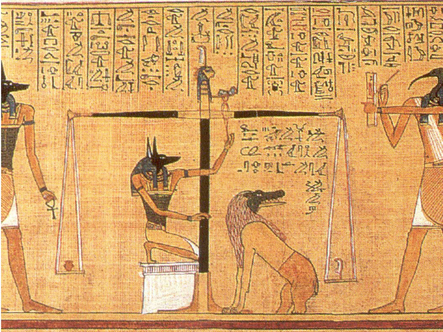
The history of balance scales begins in ancient Egypt, possibly as far back as 5000 BCE. The Egyptians used balance scales to compare the weights of goods. They placed goods on each side of the scale; when the scale became balanced, they knew that the weights of the goods were equal.
- What type of scales have you used, or seen someone else use, to measure things?
- How are the scales you've used similar to, or different from, the balance scale?
- Think about places you visit, like the grocery store or the doctor's office. Have you seen scales there?
- Scales are used to measure weight. What are some of the things we weigh?
Have students look at the Balancing the Scale interactive. Demonstrate how to put 2 and 3 on the left side of the scale.
Ask students: What number(s) do you need to place on the right side of the scale in order to balance the scale? Have students turn and talk to their partners about the question, and then try to balance the scale. After a few minutes, have students share and discuss their findings with the class. When several responses have been verbalized, discuss the definition of equation. Then ask students to represent the balance scale using an equation.
Ask students: How can you make the scale unbalanced so that the left side is heavier than the right side? Have students unbalance the scale and share what they did. Then discuss the definition of inequality. Ask students to represent the unbalanced scale using an inequality.
Possible Answers
- 5; 4 and 1; or 2 and 3
- 2 + 3 = 5; 2 + 3 = 4 + 1; or 2 + 3 = 2 + 3
- Answers will vary.
- Possible answer: 2 + 3 > 3
Balance Scales
- An equation consists of two equivalent expressions that are linked by an equal sign (=).
- An inequality consists of two nonequivalent expressions that are linked by a less than sign (<) or a greater than sign (>).
Using the Balance Scale interactive, place the numbers 2 and 3 on the left side of the scale.
- What number(s) do you need to place on the right side of the scale in order to balance the scale?
- Write an equation to represent the balanced scale.
- Now, “unbalance” the scale so that what is on the left side is greater than what is on the right side.
- Write an inequality to represent the unbalanced scale.
INTERACTIVE: Balancing the Scale
Math Mission
Discuss the Math Mission. Students will set up balanced and unbalanced scales and represent the scales using equations and inequalities.
Set up balanced and unbalanced scales, and represent the scales using equations and inequalities.
Equations and Inequalities
Have students work in pairs on these problems.
ELL: For this task, encourage students to explain their ideas to one another. Math language must be used. Encourage the use of English without discouraging students from using their primary language.
Mathematical Practices
Mathematical Practice 7: Look for and make use of structure.
Look for students who have ideas that help them relate the equal sign (=) and the inequality symbols (< and >) to the tilt of the scale.
Interventions
Student does not understand the task.
- Reread the instructions. Ask your partner for help.
- What does a balanced scale look like?
- What does an unbalanced scale look like?
Student does not know how to write an equation or an inequality to represent the scale.
- What is the value of the left side of the scale? The right side?
- Is the scale balanced or unbalanced?
- What sign can you use to represent a balanced scale?
- What symbols can you use to represent an unbalanced scale?
- What does the < symbol mean?
- What does the > symbol mean?
Student has a solution.
- Explain your strategy for setting up the balance scale.
- Explain how your equation [inequality] represents your balance scale.
SWDL Check for understanding by asking students to restate new terms or concepts in their own words, as well as any directions they will need to follow during the lesson. Students should be able to explain the relationship between a balanced equation and an unbalanced inequality.
- Answers will vary. A balanced scale that has two numbers on each side, using four different numbers: 1 + 5 = 2 + 4
- A modified scale from the previous step with the right side less than the left side: 1 + 5 > 1 + 4
- An unbalanced scale with one number on one side and two numbers on the other side: 6 > 2 + 1
- A modified scale from the previous step that is balanced: 6 = 5 + 1
- An unbalanced scale that has three numbers on one side and two numbers on the other side, such that the side with the two numbers is greater than the side with the three numbers: 1 + 2 + 3 < 4 + 5
- A modified scale from the previous step that is balanced: 1 + 2 + 3 = 1 + 5
- A modified scale from the previous step that has the same number added on each side: 1 + 2 + 3 + 4 = 1 + 5 + 4. The scale remains balanced after placing the same number on each side.
Set up numbers on both sides of the scale to match the descriptions below. After you set up each scale, write the equation or inequality that represents the scale.
- Use Balance Scale A to set up a balanced scale (both sides equal) that has two numbers on both sides, using four different numbers.
- Modify your scale from the previous step to make the right side less than the left side.
- Use Balance Scale B to set up an unbalanced scale with one number on one side and two numbers on the other side.
- Modify your scale from the previous step to make it balanced.
- Use Balance Scale C to set up an unbalanced scale that has three numbers on one side and two numbers on the other side, such that the side with two numbers is greater than the side with the three numbers.
- Modify your scale again by placing the same number on both sides. What happens?
INTERACTIVE: Balance Scale A
INTERACTIVE: Balance Scale B
INTERACTIVE: Balance Scale C
- If the scale is balanced, write an equation.
- If the scale is not balanced, write an inequality.
Prepare a Presentation
Preparing for ways of thinking.
Look for students who understand that a balanced scale can be represented with an equation and an unbalanced scale can be represented with an inequality statement. Identify different solutions to share in the Ways of Thinking discussion. Make note of students who are having trouble so you can address any misconceptions in the Ways of Thinking discussion.
- Presentations will vary.
Challenge Problem
The Challenge Problem reuses the interactive Balance Scale B. Instruct students to ignore the directions in the interactive, and to use the scale to complete the directions given in the Challenge Problem.
- No, if you add the same amount to each side of an unbalanced scale, the scale will remain unbalanced.
- Choose one equation or inequality that you created in the Balance Scale interactives that you think is particularly interesting.
- Use this equation/inequality to explain your understanding of equations and/or inequalities. In your explanation, refer to the corresponding scale you created using the interactive.
NOTE: Ignore the instructions in the interactive and follow the steps below.
- Place a number on the left side of the scale.
- Place a different number on the right side.
- Is there any one number you can now add on both sides that will balance the scale? Explain.
- An equation consists of two equivalent expressions that are linked by an equal sign.
Make Connections
Have students share their presentations. Review the following points as students share their work:
- Point out different ways students set up a balanced scale that has two numbers on each side, using four different numbers. Ask students why each representation of the scale uses an equation.
- Discuss the different ways students modified the scale to make the right side less than the left side. Some students may have added to the left side, while others may have taken away from the right side. Compare the different inequality statements that represent these approaches. Why do they all use the > symbol?
- Look for different ways of setting up an unbalanced scale with one number on one side and two numbers on the other side. Some students may have the one number greater than the two numbers; other students may have the one number less than the two numbers. Discuss the different inequality statements and how they represent the unbalanced scales. Have students who have devised a way of knowing which inequality symbol to use share their strategies.
- Then discuss how to make an unbalanced scale balanced. What do you need to do to make a scale balanced? Students may have added to one side or taken away from a side. Compare the different representations of the balanced scale. What is similar? (They all use an equal sign.)
- Then have students compare different strategies for finding two numbers that are greater than three numbers and how the unbalanced scale is represented using an inequality statement.
- Be sure at the end of the discussion that students understand the meanings of equation and inequality and how they are modeled using a scale.
Have students who completed the Challenge Problem explain why it is impossible to add the same number to each side of an unbalanced scale to balance the scale. Demonstrate using the Balance Scale B interactive.
ELL: When selecting a group of students to present in the Ways of Thinking section, ensure students present a topic they are confident about. Have students draw diagrams or demonstrate their knowledge in some other way than through verbal language alone.
Performance Task
Ways of thinking: make connections.
Take notes as your classmates explain their understanding of equations and inequalities.
As your classmates present, ask questions such as:
- Should the pointed side of the inequality sign point to the greater or lesser number?
- How does the equation or inequality you wrote represent the balance scale you made?
- What can you do to an unbalanced scale to balance it? How can you represent the balanced scale using an equation or an inequality?
- What can you do to a balanced scale to make the right side greater than the left side? How can you represent this scale using an equation or an inequality?
Equal to, Greater Than, or Less Than?
As students complete these problems, look for students who may be struggling with fraction and decimal concepts, operations, or negative numbers. Pair those students with students who have been successful with these concepts.
SWD: Students with disabilities may have difficulty working with decimals and fractions, especially when applying decimals and fractions to inequalities. If students demonstrate difficulty to the point of frustration, provide direct instruction on the basics for adding decimals and fractions.
Mathematics
As you go over the answers to these problems, encourage students who used mathematical reasoning, properties, or estimation to share their thinking processes.
For example:
- For 5 + 7 ☐ 8 + 12, I saw immediately that 5 + 7 was 12, so 8 + 12 must be greater. Therefore, 5 + 7 < 8 + 12.
- For 1 3 ☐ 1 5 , I knew that if a whole were divided into 3 pieces, each piece would be greater than if that whole were divided into 5 pieces. Therefore, 1 3 > 1 5 .
- For 5.4 + 2.06 ☐ 8 + 0.3, I knew the left side was less than 8, so it had to be less than the right side. Therefore, 5.4 + 2.06 < 8 + 0.3.
- For 9.8 + 6.7 + 0.4 ☐ 6.7 + 9.8 + 0.4, I knew that the two expressions were equal because of the commutative property of addition. Therefore, 9.8 + 6.7 + 0.4 = 6.7 + 9.8 + 0.4.
- For 1 2 ☐ 1 4 + 1 3 , I knew that 1 2 = 1 4 + 1 4 , and I knew 1 3 was greater than 1 4 . Therefore, 1 2 < 1 4 + 1 3 .
a. = b. < c. > d. < e. = f. < g. = h. < i. < j. >
- Place =, >, or < in the boxes in the equations and inequalities.
INTERACTIVE: Equal to, Greater Than, or Less Than?
A Possible Summary
A statement that shows that two expressions are equal to one another is an equation. You can use an equal sign (=) to show that the expressions are equal. A statement that shows that two expressions are unequal is an inequality statement; an inequality statement specifies which expression has the greater value (or lesser value). You can use the less than (<) or greater than (>) symbols to show which expression is less than or greater than the other.
Formative Assessment
Summary of the math: equations and inequalities.
Write a summary about equations and inequalities based on what you learned today.
Check your summary:
- Do you explain the difference between an equation and an inequality?
- Do you explain the meaning of the signs <, >, and =?
Reflect On Your Work
Have each student write a quick reflection before the end of the class. Review the reflections to learn if students understand how equations and inequalities can be represented using a balance scale.
Write a reflection about the ideas discussed in class today. Use the sentence starter below if you find it to be helpful.
A balance scale helps me understand equations and inequalities because …
abstractmath.org 2.0 help with abstract math
THE SYMBOLIC LANGUAGE OF MATH
Symbolic expressions, reading symbolic expressions, images and metaphors for symbolic expressions, grammar of the symbolic language, variables and substitution, variable objects, other symbols.
The symbolic language of math is a distinct special-purpose language. Unlike mathematical English , it is not a variety of English. It has its own rules of grammar that are quite different from those of English. You can usually read expressions in the symbolic language in any math article written in any language.
This chapter discusses aspects of the symbolic language that may cause difficulties to newcomers. It is not a systematic introduction to the symbolic language. You can find more information in the links in The languages of math.
Warning: The terminology used here to talk about symbolic expressions is nonstandard. See Variations in terminology for more detail.
The chapter More about the languages of math discusses topics that involve both the symbolic language and mathematical English.
The symbolic language consists of symbolic expressions written in the way mathematicians traditionally write them.
A symbolic expression consists of symbols arranged according to specific rules. Every symbolic expression is one of two types: symbolic assertion and symbolic term.
Every expression in the symbolic language is either a symbolic assertion or a symbolic term .
Symbolic assertions
A symbolic assertion is a complete statement that stands alone as a sentence .
A symbolic assertion says something.
- Symbolic assertions play the same role in the symbolic language as assertions do in math English .
- A symbolic assertion may contain variables and it may be true for some values of the variables and false for others.
- "$\pi\gt0$" is a symbolic assertion. It is true.
- "$\pi=3$" is a symbolic assertion. It is false, but it is nevertheless a symbolic assertion.
- "$x\gt0$" is true for $x=42$ and many other numbers and false for $x=-.233$ and many other numbers.
- The symbolic assertion "$x^2-x-2=0$" is true for the numbers $x=-1$ and $x=2$, but not for any other number.
- "$x^2-y^2=(x-y)(x+y)$" is a symbolic assertion with two variables. It is true for all numbers $x$ and $y$. Such a thing is commonly called an algebraic identity or identity relation .
- The assertion "$x^2\geq0$" is true for all real numbers, but not for all complex numbers. So the data type of a variable matters in determining whether an assertion containing the variable is always true or not.
- The assertion "$x^2\lt0$" is false for all real numbers.
- The assertion "${{x}^{2}}-6x+4y\gt0$" is true for some values of $x$ and $y$ and false for others. For example, it is false for $x=1$ and $y = 0$ and true for $x= 1$ and $y = 2$. There is more about symbolic assertions like this one in the section on constraints
Symbolic statements
A symbolic statement is a symbolic assertion without variables.
- A symbolic statement is either true or false.
- A symbolic statement is regarded as a special case of a symbolic assertion. What makes it special is that it contains no variables.
- $\pi\gt0$ and $3^2=9$ are true symbolic statements.
- $\pi\lt0$ and $2+3=6$ are false symbolic statements. Even though false, they are still regarded as symbolic statements.
Symbolic terms
A symbolic term is a symbolic expression that refers to some mathematical object.
A symbolic term names something.
Terms play the same role in the symbolic language that descriptions do in math English.
- The expression “${{3}^{2}}$” is a symbolic term . It is another name for the number $9$.
- "$x^2$" is a symbolic term containing a variable $x$. This means the term has variable meaning depending on which value is substituted for $x$. For example, if you set $x=-2$, you get $(-2)^2$, another name for $4$.
- ${{x}^{2}}-6x+4y$ (mentioned above) is symbolic term with two variables. If you substitute $2$ for $x$ and $3$ for $y$ then the expression denotes the integer $4$.
Variations in terminology
The names “symbolic assertion” and “symbolic term” are not standard usage in math . In mathematical logic:
- Symbolic assertions may be called formulas or predicates.
- True assertions may be called propositions or sentences .
All these words, as well as my use of “ term ”, can cause cognitive dissonance:
- Many people would refer to “${{\text{H}}_{\text{2}}}\text{O}$” as “the formula for water”, but it is not a formula in sense of logic because it does not make a statement.
- In everyday usage “proposition” may mean a statement to be debated, or a proposal for action, but in math logic the meaning is simply a statement .
- The name “ term ” comes from mathematical logic. The expression “${{x}^{3}}\left( {{y}^{2}}-1 \right)$” contains symbolic terms ${{x}^{3}}$ and ${{y}^{2}}-1$, which would in math English be called factors rather than "terms".
| This kind of conflict between different parts of math |
Non-algebraic expressions
Symbolic expressions don’t have to have algebraic form and they do not have to name numbers.
- Texts on group theory use the expression " ${{\text{S}}_{n}}$ " to denote the group of all permutations of an $n$-element set, with composition as operation.
- The group ${{\text{S}}_{3}}$ contains six elements. You can write them out and make a table of the group multiplication (described here ).
- All true statements about ${{\text{S}}_{3}}$ are implied by the symbol.
- Operations can be performed on groups, just as they can for numbers. One operation is the product of two groups . In particular one can form the product ${{\text{S}}_{n}}\times\mathbb{Z}/3$. ( $\mathbb{Z}/3$ is another group.) This is a symbolic term just like "$a\times b$", but in group theory rather than in elementary algebra.
Each branch of mathematics is concerned with certain particular kinds of mathematical objects, and every one of them studies many different kinds of operations on the objects , expressed (usually) in symbolic notation.
Distinguish between assertions and terms
A fundamental difficulty many people new to algebra have is that they don't pay attention to the difference betweeen assertions and terms.
An expression such as “$x\alpha y$, where $\alpha$ is any old symbol, may be an assertion ( saying something) or a term ( naming something).
- “$x \lt y$” is an assertion – a complete statement. If $x$ and $y$ have specific real number values, then the statement is either true or false.
- “$x+y$” is a term – an expression to be evaluated. For this expression, if you plug in $x=2$ and $y=3$ then it names the number $5$. See encapsulated computation below.
- To write "If $x\lt y$, then $x\lt y+1$" is the same same as saying, "If $x$ is less than $y$, then $x$ is less than $y+1$". Not only is it OK to say it, it's true.
- To say "If $x+y$ then $x\lt x+y$" is nonsense. The expression "$x+y$" is not a sentence and so can't be a clause after "if". In the same way, it is nonsense to say "If my house, then it is white".
Division and fractions
Two symbols used in the study of integers are notorious for their confusing similarity.
- The expression "$m/n$" is a term denoting the number obtained by dividing $m$ by $n$. Thus "$12/3$" denotes $4$ and "$12/5$" denotes the number $2.4$.
- The expression "$m|n$" is the assertion that "$m$ divides $n$ with no remainder". So for example "$3|12$", read "$3$ divides $12$" or "$12$ is a multiple of $3$", is a true statement and "$5|12$" is a false statement.
Notice that $m/n$ is an integer if and only if $n|m$. Not only is $m/n$ a number and $n|m$ a statement , but the statement "one is an integer if and only if the other is true" is correct only after the $m$ and $n$ are switched!
| It is wise to be a bit paranoid |
When you see a complicated assertion or term you have to be patient . You must stop and unwind it. Read the tiresomely long example of unwinding an expression in Zooming and Chunking.
Giving names to symbolic expressions
Turning symbolic terms into functions.
The expression "${{x}^{2}}-1$" is a symbolic term. You may define a function $f$ whose value at $x$ is given by the expression ${{x}^{2}}-1$. After we say that, "$f$" is a name for the function.
See Functions: images and metaphors.
Naming assertions
You can also give names to symbolic assertions.
- Let $P(x)$ be the expression “$x\gt1$”. In this case, you could write statements such as “$P(3)$ is true” and “$P(1/2)$ is false", as well as more complicated statements such as "For any number $x$, if $P(x)$ then $x\gt0$."
- Don’t let this notation mislead you into thinking “$P(3)$” is a number. “$P(3)$” is a statement, namely the statement “$3\gt1$”. Of course, $P$ may be thought of as a function $f:\mathbb{R}\to \{\text{true, false}\}$.
Using notation such as “$P(x)$” for statements occurs mostly but not entirely in texts on logic. (This claim needs lexicographical research.) An overview of its use in first-order logic is given in Mathematical reasoning. See also the Wikipedia articles on various kinds of logic:
- First-order logic
- Intuitionistic logic
- Type theory
Symbolic terms are encapsulated computations
Algebraic terms are encapsulated computations.
| A symbolic expression in algebra is both of these things: |
If you are fairly proficient in algebra, you already know this subconsciously about algebraic expressions.
- The expression “$2\cdot 2+3$” is both a name for the number $7$ and a description of a particular calculation that gives $7$.
- In the math ed literature, we say that the expression “$2\cdot 2+3$” encapsulates the process of multiplying $2$ by itself and adding $3$. See the article What is the object of the encapsulation of a process? .
- The expression “$63/9$” is also a name for the number $7$ and encapsulates a different calculation that results in $7$.
- It encapsulates a proper-name calculation, because in our culture “$7$” is the default symbolic name of the number.
- A proper-name calculation is like referring to "Henry" in a conversation where those present know which Henry you are talking about.
- In the case of $7$, the context is that we are talking about math, where everyone is supposed to know what the symbol "$7$" means.
- The expression “$371$” is our default name for $371$. It is in decimal notation and encapsulates the calculation “$3\cdot 100+7\cdot 10+1$”.
- The expression “The largest positive root of ${{x}^{3}}-9{{x}^{2}}+15x-7$” is a name for $7$, but that fact requires a more difficult calculation that $2\cdot 2+3$ or $63/9$. Indeed, you don’t even know that the expression is a correctly formed name of a number until you work out that ${{x}^{3}}-9{{x}^{2}}+15x-7$ has a positive root.
- The expression \[3{{x}^{2}}-2x-5\] names a variable number . Like most variable mathematical objects, some statements about it must be said to be neither true nor false. For example, "$3{{x}^{2}}-2x-5\leq12$" is neither true nor false. On the other hand, it is a nice calculus exercise to show that “$3{{x}^{2}}-2x-5\le -6$” is definitely false for any $x$.
Most math objects can be combined into new constructions, making expressions like algebraic expressions except that the variables represent structures or objects instead of numbers. Groups, various kinds of spaces, and lots of math objects you never heard of can be combined into "products" and "coproducts", and many of them have "quotients", "function spaces" and other constructions. Most Wikipedia articles about important kinds of math objects describe some of these constructions. The expressions representing such things can still be thought of as both an encapsulated computation and as the name of another math object.
Symbolic expressions as trees
Symbolic expressions such as "$4(x-2)=3$" and the very similar looking "$4x-2=3$" have different abstract structures. The difference results in different solutions: $x=11/4$ and $x=5/4$ respectively. The abstract structures are largely invisible, with the only hint about the difference being the presence or absence of parentheses.
There are other ways to exhibit symbolic expressions that make the abstract structure much more obvious. One way is to use trees . Examples of the tree representation of expressions are given in the following posts in Gyre&Gimble:
- Presenting binops as trees
- The only axiom of algebra
- A visualization of a computation in tree form
I expect to include examples like these in a future revision of this article.
Arrangement of symbols is meaningful
In symbolic expressions, the symbols and the arrangement of the symbols both communicate meaning.
- “${{\sin }^{2}}x$” , “$\sin 2x$” and “$2\sin x$” all mean different things.
- “$x{{2}^{\sin }}$” is meaningless.
- “${{\sin }^{2}}x$” and “${{\left( \sin x \right)}^{2}}$” mean the same thing . If you took a class in precalculus or calculus, you may have had this fact expressed explicitly or you may have learned it by osmosis (see “osmosis theory” in the Handbook .).
Subexpressions
An expression may contain several subexpression s . The rules for forming expressions and the use of delimiters let you determine the subexpressions.
- The subexpressions in “${{x}^{2}}$” are “ x” and “$2$”.
- The subexpressions in “${{(2x+5)}^{3}}$” are "$2$", "$x$", “$2x$”, "$5$", “$2x+5$” and "$3$".
Math English subexpressions
A phrase in math English can be a subexpression of a symbolic expression.
- The set $\left\{ {{n}^{3}}|n\in \mathrm{}\text{, }n\gt0 \right\}$ could also be written as$\left\{ {{n}^{3}}|n\text{ is a positive integer} \right\}$.
Embedded symbolic expressions in math English
Symbolic expressions in texts are usually embedded in sentences in math English, although they may stand independently.
- "If $x\lt y$, then $x\lt y+1$." This math English sentence occurred earlier in this chapter.
- "The indefinite integral of the function $x^2+1$ is $\frac{x^3}{3}+x+C$, where $C$ is an arbitrary real number."
- The statement "$\int (x^2+1)dx=\frac{x^3}{3}+x+C$" could occur in a text by itself as a sentence, but that is uncommon except perhaps in lists.
Embedded symbolic expressions in math English involves a remarkable number of subtleties. Teachers almost never tell you about these subtleties. The abstractmath article Embedding reveals a few of these secrets. Generally, students learn these facts unconsciously. Some don't, and those generally don't become math majors.
The expression $xy+z$ means $(xy)+z$, not $x(y+z)$. This is an illustration of the principle that in an algebraic expression, multiplication is performed first, then addition . We say multiplication has a higher precedence that addition.
When two operations have the same precedence, the operations should be done from left to right. The mnemonic “Please Excuse My Dear Aunt Sally” (PEMDAS) describes the order of the common operations:
- Parentheses (calculate what is inside the parentheses before you do anything alse.)
- Exponentiation
- Multiplication and Division
- Addition and Subtraction.
One more rule
The names of functions of one variable generally have the highest precedence, except for unary minus , which has lowest precedent.
- "$2\cdot 3+5$" means do the multiplication first, then add the five, getting 11, whereas "$2\cdot (3+5)$" means do the addition first, then multiply the result by $2$, getting $16$.
- "$4+3^2$" means first calculate $3^2=9$, getting $4+9$, then calculate $4+9$, getting $13$. But $(4+3)^2$ means $7^2$.
- The expression "$\sin x+y$" means calculate $\sin x$ and add $y$ to the result. The expression "$\sin(x+y)$" means calculate $x+y$, then take the sine of the result.
- $-{{3}^{2}}$ requires you to calculate ${{3}^{2}}$ first, then apply the minus sign, yielding $-9$. On the other hand, ${{(-3)}^{2}}$ yields $9$.
- Because so many people new to math misread some of these expressions, I have acquired the habit of putting in theoretically unnecessary parentheses for clarity. So for example I would write $(\sin x)+y$ instead of $\sin x+y$ and $-({{3}^{2}})$ instead of $-{{3}^{2}}$.
- There is supposed to be a rule that says that ${{2}^{{{x}^{\,y}}}}$ denotes $2{{\,}^{\left( {{x}^{\,y}} \right)}}$, but this is even more widely unknown, so I always write $2{{\,}^{\left( {{x}^{\,y}} \right)}}$.
- But note: ${{({{2}^{x}})}^{\,y}}={{2}^{x\,y}}$, which is not usually equal to $2{{\,}^{\left( {{x}^{\,y}} \right)}}$ .
- Wikipedia has an excellent detailed description of the precedence rules of algebra.
Irregular syntax in the symbolic language
The symbolic language of math has developed over the centuries the way natural languages do. In particular, the symbolic language, like English, has definite rules and it has irregularities.
In English, the plural of a noun is normally formed by adding “s” or “es” according to fairly precise rules. (The plural of car is cars, the plural of loss is losses.)
But English rules have exceptions . Think mouse/mice (instead of mouses) and hold/held (instead of holded for the past tense). .
The symbolic language of math has a lot of rules too. In the symbolic language, the symbol for a function is usually put to the left of the input ( argument ) and the input is put in parentheses. For example if $f$ is the function defined by $f(x)=x+1$, then the value of $f$ at $3$ is denoted by $f(3)$ (which of course evaluates to $4$.)
Irregularities
Just as English has irregular plurals and past tenses, the symbolic language has irregular syntax for certain expressions. Here are two of many examples of irregularities.
- The symbol “!” for the factorial ( MW , Wi ) function is put after the argument. For example, $6! = 720$.
- The parentheses around the argument of a function are omitted for the trig and log ( MW , Wi ) functions, so we typically write $\sin x$ instead of $\sin(x)$ and $\log x$ instead of $\log(x)$. More about that here.
There are many other examples of irregularities in symbolic notation in these places:
- Notation for the value of a function
- Variations in meaning
- The Handbook (search for "Irregular syntax").
Other sections of this chapter are in separate files:
This work is licensed under a Creative Commons Attribution-ShareAlike 2.5 License .
- Skip to main content
Welcome, Fellow Math Enthusiast! I’m so happy you’re here!
- Counting & Cardinality
- Addition & Subtraction
- Multiplication & Division
- Place Value & Base Ten
- Measurement & Data
- Geometry & Fractions
- Vocabulary & Discourse
- Math Manipulatives
- Classroom Management
- Classroom Organization
- Holidays & Seasonal
- Social-Emotional Learning
- Privacy Policy
- Terms of Use
- SHOP RESOURCES
- BECOME A MEMBER
- Search this website
Teaching with Jillian Starr
teaching little stars to shine brightly
FREE Number Talks
First grade teachers, access 20 FREE Number Talk Prompts to enhance your place value unit and get your students engaged in conversation.
Mathematical Representations Series Part 4: Verbal Representation

Welcome back to our deep dive into mathematical representations! Today, we are taking a look at symbolic representations and how we can translate between symbolic, concrete, and visual representations. First, let’s do a two-sentence recap of this series so far:
We have already focused on concrete representations and the immense value of manipulatives, the range of visual representations we want to encourage with our students, and how we can use numerals and operations to represent thinking symbolically . We are centering our conversation around Lesh’s Translation Model, which encompasses the range of ways we represent our thinking, and stresses the importance of making connections between representations.
Today we are talking about verbal representations. While it’s an essential form of representation for our students, it is often less discussed. This is likely due to the fact that it is not explicitly called out in the Concrete-Pictorial Abstract model . This is just another reason why I love introducing teachers to Lesh’s translation model alongside the CPA (often called CRA) model.
Verbal Representation
The language we use to communicate our thoughts and ideas is another equally important representation. This can be oral, written, signed, or any way that a student would look to communicate language. James Heddens writes that students “need to be given opportunities to verbalize their thought processes: verbal interaction with peers will help learners clarify their own thinking.”
If we go back to our previous examples from concrete, visual, and abstract thinking, we have a student with five yellow counters and four red counters. The student then sketched their counters and wrote the number sentence 5+4=9 on their paper.

So how does verbal representation come into play? Perhaps after the activity, a student shows you their sketch of the counters. When you ask them about their drawing, they may share “I had nine counters. Four of them were red and five of them were yellow, and that makes nine.” That statement is a verbal representation of the concept. They have also just translated their visual representation to a verbal representation.
Connecting Two Verbal Representations
If wanted, we could take it a step further by asking the student to write their thoughts down. This will require the student to revisit their thoughts communicated orally and condense them into a written description, like “Four counters and five counters make nine counters.” This extra step of condensing their language into a second form, allowed students to connect two verbal representations. WOW!

Verbal representation is essential to our work, especially in the early grades. Our students who may not have the ability to write words or numbers will often communicate their understanding orally. This NEEDS to be a part of the discussion when we talk about deepening student understanding, and it’s a huge reason why I make sure to consider Lesh’s Translation Model in addition to the Concrete-Pictorial-Abstract model.
What’s Up Next?
This series is going to dive deep into each of the representations discussed in Lesh’s Translation Model, and then we are going to put it all together so we can make a big impact on your math teaching this year.
If you missed Part One about Concrete Representations , Part Two about Visual Representations , or Part Three about Symbolic Representations , check them out so you have all of the info you need before we move on!
Math Vocabulary Resources

You May Also Enjoy These Posts:
Reader Interactions
Leave a comment.
Your email address will not be published. Required fields are marked *
This site uses Akismet to reduce spam. Learn how your comment data is processed .

Ready to go deeper?
JOIN MEANINGFUL MATH

hello I'm Jillian
I’m so happy you’re here. I want every child to feel confident in their math abilities, and that happens when every teacher feels confident in their ability to teach math.
In my fifteen years of teaching, I sought every opportunity to learn more about teaching math. I wanted to know HOW students develop math concepts, just like I had been taught how students learn to read. I want every teacher to experience the same math transformation I did, and have the confidence to teach any student that steps foot in their classroom. I’m excited to be alongside you in your math journey!
Follow Me on Instagram!

Writing the Symbolic Representation of a Function (Graph → Symbolic)
Let's get started.
You will learn to represent functions in different forms and use your graphing calculator to find equations that match different graphs.
TEKS Standards and Student Expectations
A(2) Linear functions, equations, and inequalities. The student applies the mathematical process standards when using properties of linear functions to write and represent in multiple ways, with and without technology, linear equations, inequalities, and systems of equations. The student is expected to:
A(2)(C) write linear equations in two variables given a table of values, a graph, and a verbal description
A(7) Quadratic functions and equations. The student applies the mathematical process standards when using graphs of quadratic functions and their related transformations to represent in multiple ways and determine, with and without technology, the solutions to equations. The student is expected to:
A(7)(A) graph quadratic functions on the coordinate plane and use the graph to identify key attributes, if possible, including x -intercept, y -intercept, zeros, maximum value, minimum values, vertex, and the equation of the axis of symmetry
Resource Objective(s)
Given the graph of a linear or quadratic function, the student will write the symbolic representation of the function.
Essential Questions
What are the different forms of linear functions?
How can a graphing calculator be used to match a graph to a linear equation?
How is a quadratic equation different from a linear equation?
- Linear Function
- Quadratic Equation
Slope-Intercept Form
Introduction.
This table shows the three different ways to represent linear functions .
| slope-intercept form | = m + b |
| point-slope form | – = m( – ) |
| standard form | A – B = C |
We’ll first look at slope-intercept form . Remember that the slope is the rise over the run (i.e., the change in y -value over the change in x -value.)

To review slope-intercept form, use this linked interactive activity . Move the sliders one at a time to change the slope (the y -intercept). After you have experimented with the activity, answer the questions below.
Using a Calculator with Slope-Intercept Form
Even the best mathematicians need ways to check their work. We’re going to use the graphing calculator to make sure we have the correct answer.
If you need a graphing calculator, you can use an online calculator here .
Which equation best describes the following graph?

If you are not sure of the answer, you can use your calculator three different ways to double check. You should learn all three methods because there will be times when one of the methods will not be obvious.
We will try option C: y = 3/4 x + 5.
Method 1: Match the Graph
You can use your graphing calculator to look at a graph of an equation by following these steps:
- Enter the equation.
- Graph the equation.

The graph on the calculator looks similar to the given graph, but we can’t be sure. We certainly can tell the line is increasing. Options A and B are definitely wrong because they have a negative slope.
Method 2: Match the Graph to the Table
You can also use your graphing calculator to match the table of values from an equation by following these steps:
- Go to Y=.
- Use 2nd Graph to view the table.

You can see that the two points (0, 5) and (4, 8) are on the line and in the table.
Method 3: Match Points on a Graph Using TRACE
You can also use the graphing calculator to find points on the line using the following steps:
- Press the TRACE button and type x -values that are on the line.
We can see that the point (-4, 2) is on the graph, so we'll use the TRACE button to find where x equals -4.

The point is on the line. Just to be sure, we will try another point at (-8, -1)

This point is also on the line. Now we know that option C is correct.
Standard Form Equations and Practice
What if the equation is not in slope-intercept form? This is a standard form equation.
Ax + By = C
You can manipulate the equation, so you can use the graphing calculator to check your answer .
Forms of Linear Equations
To change a standard form equation to a slope-intercept form, you must isolate the variable y on the left side of the equation.
You can review the steps to change an equation from standard form to slope-intercept form in these 2 examples.
Example 1: Standard form to slope-intercept form .
Example 2: Standard form to slope-intercept form .
The following is a typical question you might see that has answer choices in standard form.
Which equation best describes the graph shown below?

A ) x - 2 y = 14 B ) x - 2 y = - 14 C ) x + 2 y = 14 D ) x + 2 y = - 14
Solving each equation for y , the equations are:
A ) y = 1 2 x - 7 B ) y = 1 2 x + 7 C ) y = - 1 2 x + 7 D ) y = - 1 2 x - 7
It seems that the right equation is option B .
When we enter the equation in to the graphing calculator under Y=, we see the following results.

According to this, the points (0, 7), (2, 8) (4, 9) and (6, 10) should all be points on the graph. To check this, we substitute the x - and y -values from these points into x − 2 y = −14.

We know B is correct!
Here is how you know an answer is wrong:
Option D is incorrect because the points (0, 7), (2, 8) (4, 9) and (6, 10) will not satisfy the equation x + 2 y = −14.

Quadratic Functions and Practice
Next we will look at writing equations for quadratic functions. This is the form of a quadratic function.
y = a x 2 + b x + c
Quadratic functions are parabolas and either have a U-shape or a mountain shape. Parabolas with a positive "a" value have a U-shape, and those with a negative "a" value have a mountain shape.
In addition, you know how to use a calculator to check for the correct answer, so you can input these equations in the equation editor (Y=) as well.
Which quadratic equation best represents the parabola shown below?

You can test each of the answer choices by using your graphing calculator to eliminate obviously wrong answers.
- Enter the equation in Y=.
Each graph looks like this.

Options C and D are obviously wrong because they are facing down.
Now we can look at the table values for the remaining graphs. The graph we were given contains the points (-2, 9), (-1, 6), (0, 5), (1, 6), and (2, 9). Use the TABLE.

Now you can confidently pick option B as your answer.
Remember, you can also use the TRACE key to check points on the graph. Press TRACE, type in the x -value, and press ENTER.

Vocabulary Activity
Journal activity.
Copy and paste the link code above.
Related Items
Mathematical Representations
- Living reference work entry
- First Online: 28 July 2018
- Cite this living reference work entry

- Gerald A. Goldin 2
332 Accesses
2 Citations
Definitions
As most commonly interpreted in education, mathematical representations are visible or tangible productions – such as diagrams, number lines, graphs, arrangements of concrete objects or manipulatives, physical models, written words, mathematical expressions, formulas and equations, or depictions on the screen of a computer or calculator – that encode, stand for, or embody mathematical ideas or relationships. Such a production is sometimes called an inscription when the intent is to focus on a specific instance without referring, even tacitly, to any interpretation of it. To call something a representation thus includes reference to some meaning or signification it is taken to have. Such representations are called external – i.e., they are external to the individual who produced them and accessible to others for observation, discussion, interpretation, and/or manipulation. Spoken language, interjections, gestures, facial expressions, movements, and postures may sometimes...
This is a preview of subscription content, log in via an institution to check access.
Access this chapter
Institutional subscriptions
Anderson C, Scheuer N, Pérez Echeverría MP, Teubal EV (eds) (2009) Representational systems and practices as learning tools. Sense, Rotterdam
Google Scholar
Bruner JS (1966) Toward a theory of instruction. The Belknap Press – Harvard University Press, Cambridge, MA
Common Core State Standards Initiative (2018) Preparing America’s students for success. Retrieved June 2018 from http://www.corestandards.org/
Cuoco AA, Curcio FR (2001) The roles of representation in school mathematics: NCTM 2001 yearbook. National Council of Teachers of Mathematics, Reston
Davis RB (1984) Learning mathematics: the cognitive science approach to mathematics education. Ablex, Norwood
Duval R (2006) A cognitive analysis of problems of comprehension in a learning of mathematics. Educ Stud Math 61:103–131
Article Google Scholar
Goldin GA (1998) Representational systems, learning, and problem solving in mathematics. J Math Behav 17:137–165
Goldin GA (2008) Perspectives on representation in mathematical learning and problem solving. In: English LD (ed) Handbook of international research in mathematics education, 2nd edn. Routledge – Taylor and Francis, London, pp 176–201
Goldin GA, Janvier, C (eds) (1998) Representations and the psychology of mathematics education: parts I and II (special issues). J Math Behav 17(1 & 2)
Goldin GA, Kaput JJ (1996) A joint perspective on the idea of representation in learning and doing mathematics. In: Steffe L, Nesher P, Cobb P, Goldin GA, Greer B (eds) Theories of mathematical learning. Erlbaum, Hillsdale, pp 397–430
Gravemeijer K, Doorman M, Drijvers P (2010) Symbolizing and the development of meaning in computer-supported algebra education. In: Verschaffel L, De Corte E, de Jong T, Elen J (eds) Use of representations in reasoning and problem solving: analysis and improvement. Routledge – Taylor and Francis, London, pp 191–208
Heinze A, Star JR, Verschaffel L (2009) Flexible and adaptive use of strategies and representations in mathematics education. ZDM 41:535–540
Hitt F (ed) (2002) Representations and mathematics visualization. Departamento de Matemática Educativa del Cinvestav – IPN, México
Janvier C (ed) (1987) Problems of representation in the teaching and learning of mathematics. Erlbaum, Hillsdale
Kaput J, Noss R, Hoyles C (2002) Developing new notations for a learnable mathematics in the computational era. In: English LD (ed) Handbook of international research in mathematics education. Erlbaum, Mahwah, pp 51–75
Lesh RA, Doerr HM (eds) (2003) Beyond constructivism: models and modeling perspectives on mathematics problem solving, learning, and teaching. Erlbaum, Mahwah
McClelland JL, Mickey K, Hansen S, Yuan A, Lu Q (2016) A parallel-distributed processing approach to mathematical cognition. Manuscript, Stanford University. Retrieved June 2018 from https://stanford.edu/~jlmcc/papers/
Moreno-Armella L, Sriraman B (2010) Symbols and mediation in mathematics education. In: Sriraman B, English L (eds) Advances in mathematics education: seeking new frontiers. Springer, Berlin, pp 213–232
Moreno-Armella L, Hegedus SJ, Kaput JJ (2008) From static to dynamic mathematics: historical and representational perspectives. Educ Stud Math 68:99–111
National Council of Teachers of Mathematics (2000) Principles and standards for school mathematics. NCTM, Reston
Newell A, Simon HA (1972) Human problem solving. Prentice-Hall, Englewood Cliffs
Novack MA, Congdon EL, Hermani-Lopez N, Goldin-Meadow S (2014) From action to abstraction: using the hands to learn math. Psychol Sci 25:903–910
Palmer SE (1978) Fundamental aspects of cognitive representation. In: Rosch E, Lloyd B (eds) Cognition and categorization. Erlbaum, Hillsdale, pp 259–303
Roth W-M (ed) (2009) Mathematical representation at the interface of body and culture. Information Age, Charlotte
Skemp RR (ed) (1982) Understanding the symbolism of mathematics (special issue). Visible Language 26(3)
van Garderen D, Scheuermann A, Poch A, Murray MM (2018) Visual representation in mathematics: special education teachers’ knowledge and emphasis for instruction. Teach Educ Spec Educ 41:7–23
Download references
Author information
Authors and affiliations.
Graduate School of Education, Rutgers University, New Brunswick, NJ, USA
Gerald A. Goldin
You can also search for this author in PubMed Google Scholar
Corresponding author
Correspondence to Gerald A. Goldin .
Editor information
Editors and affiliations.
South Bank University Centre for Mathematics Education, London, United Kingdom
Steve Lerman
Section Editor information
Department of Science Teaching, The Weizmann Institute of Science, Rehovot, Israel
Ruhama Even
Rights and permissions
Reprints and permissions
Copyright information
© 2018 Springer Nature Switzerland AG
About this entry
Cite this entry.
Goldin, G.A. (2018). Mathematical Representations. In: Lerman, S. (eds) Encyclopedia of Mathematics Education. Springer, Cham. https://doi.org/10.1007/978-3-319-77487-9_103-4
Download citation
DOI : https://doi.org/10.1007/978-3-319-77487-9_103-4
Received : 15 June 2018
Accepted : 02 July 2018
Published : 28 July 2018
Publisher Name : Springer, Cham
Print ISBN : 978-3-319-77487-9
Online ISBN : 978-3-319-77487-9
eBook Packages : Springer Reference Education Reference Module Humanities and Social Sciences Reference Module Education
- Publish with us
Policies and ethics
- Find a journal
- Track your research

www.springer.com The European Mathematical Society
- StatProb Collection
- Recent changes
- Current events
- Random page
- Project talk
- Request account
- What links here
- Related changes
- Special pages
- Printable version
- Permanent link
- Page information
- View source
Mathematical symbols
2020 Mathematics Subject Classification: Primary: 03-XX Secondary: 01Axx [ MSN ][ ZBL ]
Conventional signs used for the written notation of mathematical notions and reasoning. For example, the notion "the square root of the number equal to the ratio of the length of the circumference of a circle to its diameter" is denoted briefly by $\sqrt{\pi}$, while the statement "the ratio of the length of the circumference of the circle to its diameter is greater than three and ten seventy-firsts and less than three and one seventh" is written as \[ 3 + \frac{10}{71} < \pi < 3 + \frac{1}{7}\, . \]
- 1.1 The origins
- 1.2 Ancient Greece
- 1.3 Post-Hellenistic era
- 1.4 Indian mathematics
- 1.5 Renaissance
- 2.2 Descartes
- 3.1 Leibniz and the modern notation
- 4 XIX Century
- 5 Mathematical logic and classification of symbols
- 6 The origin of some mathematical symbols
- 7 References
Early history
The development of mathematical notation was intimately bound up with the general evolution of mathematical concepts and methods.
The origins
The first mathematical symbols were signs for the depiction of numbers — ciphers , the appearance of which apparently preceded the introduction of written language. The most ancient systems of numbering (see Numbers, representations of ) — the Babylonian and the Egyptian — date back to around 3500 B.C..
Ancient Greece
The first mathematical symbols for arbitrary quantities appeared much later (from the 5th-4th centuries B.C.) in Greece. Arbitrary quantities (areas, volumes, angles) were represented by the lengths of lines and the product of two such quantities was represented by a rectangle with sides representing the respective factors. In Euclid's Elements (3th century B.C.), quantities are denoted by two letters, the initial and final letters of the corresponding segment, and sometimes by one letter. Dating from Archimedes (287–213 B.C.), the latter device became standard. This mode of notation could potentially have developed into a calculus of letters. In the mathematics of classical Antiquity, however, no operations were carried out on letters and such a letter calculus did not materialize.
Post-Hellenistic era
The rudiments of letter notation and calculus appeared in the post-Hellenistic era, thanks to the liberation of algebra from its geometric setting. Diophantus (probably 3th century A.D.) denoted the unknown $x$ and its powers by the following symbols: \[ \begin{array}{llllll} x\quad & x^2\quad & x^3\quad & x^4\quad & x^5\quad & x^6\\ \varsigma' &\delta^{\tilde{\upsilon}} &\kappa^{\tilde{\upsilon}} & \delta \delta^{\tilde{\upsilon}}&\delta \kappa^{\tilde{\upsilon}}& \kappa \kappa^{\tilde{\upsilon}} \end{array} \] ($\delta^\tilde{\upsilon}$ — from the Greek term $\delta\upsilon'\nu\alpha\mu\iota\varsigma$, denoting the square of the unknown; $\kappa^{\tilde{\upsilon}}$ — from the Greek $\kappa\upsilon'\beta\omicron\varsigma$, cube). Diophantus wrote coefficients to the right of the unknown or its powers, e.g. $3 x^5$ was denoted by $\delta \kappa^{\tilde{\upsilon}} \bar{\gamma}$ (where $\bar{\gamma} = 3$). Terms to be added together were simply juxtaposed, while subtraction required the special symbol $\wedge$; equality was denoted by the letter $\iota$ (from the Greek $\iota\sigma\omicron\varsigma$, equal). For example, Diophantus would have written the equation \[ (x^3+8x)-(5x^2+1) = x \] as follows: \[ \kappa^{\tilde{\upsilon}}\;\bar{\alpha}\;\varsigma'\; \bar{\eta}\; \bigwedge\; \delta^{\tilde{\upsilon}}\; \bar{\epsilon}\; \mu^0\; \bar{\alpha}\; \iota\; \varsigma'\;\bar{\alpha} \] (here $\bar{\alpha} =1$, $\bar{\eta}=8$, $\bar{\epsilon}=5$ and $\mu^0\bar{\alpha}$ means that the unit $\bar{\alpha}$ is not to be multiplied by a power of the unknown).
Indian mathematics
Several centuries later, the Indians, who had developed a numerical algebra, introduced various mathematical symbols for several unknowns (abbreviations for the names of colours, which denoted the unknowns), the square, the square root, and the subtrahend. Thus, the equation \[ 3 x^2 + 10x - 8 = x^2 +1 \] was written in Brahmaputra's notation (7th century) as follows:
ya va $3$ ya $10$ ru $8$
ya va $1$ ya $0$ ru $1$
(ya — from yavat — tavat, unknown; va — from varga, squared number; ru — from rupa, a rupee coin — free term; a dot above a number denotes subtraction).
Renaissance
The creation of modern algebraic symbols dates to the 14th–15th centuries; it was conditioned by achievements in practical arithmetic and the study of equations. Symbols for various operations and for powers of an unknown quantity appeared spontaneously in different countries. Many decades — sometimes centuries — elapsed until a specific symbol became accepted as convenient for calculations. Thus, at the end of the 15th century N. Chuquet and L. Pacioli (Fra Luca Pacioli) were using the symbols $p$ and $m$ (from the Latin plus and minus) for addition and subtraction, respectively, while German mathematicians introduced the modern $+$ (probably an abbreviation for the Latin et) and $-$. As late as the 17th century, one could count about ten different symbols for multiplication.
The history of the radical sign is instructive. Following Leonardo Pisano (Leonardo da Pisa) (1220), and up to the 17th century, the symbol $RR$ (from the Latin "radix", i.e. root) was widely employed for "square root" . Chuquet denoted square, cube, etc., roots by $RR^2, RR^3$, etc. In a German manuscript of ca. 1480 the square root is denoted by a dot before the number, the cube root by three dots, and the fourth root by two dots. By 1525 one can already find the symbol $\sqrt{}$ (Ch. Rudolff, sometimes written as K. Rudolff). For higher-order roots, some scholars simply repeated this symbol; others wrote a suitable letter after the symbol (an abbreviation of the name of the exponent), and still others inscribed a suitable figure in a circle or between parentheses or square brackets in order to distinguish it from the number under the radical sign (the horizontal line over the radicand was introduced by R. Descartes, 1637). Only at the beginning of the 18th century did it become customary to write the exponent above the opening of the radical sign; the first appearance of this convention, though, was much earlier (A. Girard, 1629). Thus, the evolution of the radical sign extended over almost 500 years.
Modern algebraic notation
Mathematical symbols for an unknown quantity and its powers were highly diverse. During the 16th century and early 17th century, more than ten rival notations were current for just one square of an unknown; among these were ce (from census — the Latin term serving as translation for the Greek term $\delta \upsilon'\nu\alpha\mu \iota\varsigma$), Q (for quadratum), $zz$, $\frac{ii}{1}$, A , $1^2$, $A^{ii}$, aa, $a^2$, etc. G. Cardano (1545) would have written the equation \[ x^3 + 5x = 12 \] as follows: \[ 1 .\; {\rm cubus}\, \square.\;\varsigma\; . {\rm positionibus equantur}\; 12 \] (cubus $=$ cube, positio $=$ unknown, æquantur $=$ equals).
The same equation, written by M. Stifel (1544), would have been: \[ 1+5.\; {\rm aequ}.\; 12 \] by R. Bombelli (1572): \[ 1p\; .\; 5 {\rm eguale\; a\;} 12 \] by F. Viète (1591): \[ 1C + fN,\; {\rm aequatur}\; 12 \] (C $=$ cubus $=$ cube, N $=$ numerus $=$ number);
and by T. Harriot (1631): \[ aaa+5.a=12 \] The 16th century and early 17th century saw the first appearance and use of the equality sign and brackets; square brackets (Bombelli, 1550), parentheses (N. Tartaglia, 1556), and curly brackets (Viète, 1593).
A significant step forward in the development of mathematical notation was Viète's introduction (1591) of capital letters of the Latin alphabet to denote both arbitrary constant quantities and unknowns; consonants, such as B, D, ... were reserved for constants, and vowels A, E, ... for unknowns. This made it possible for the first time to write down algebraic equations with arbitrary coefficients and to operate with them. For example, Viète's equation \[ A\, {\rm cubus}\; +\; B\, {\rm plano}\; {\rm in}\; A3\;.\; {\rm aequatur}\;D\; {\rm solido} \] (cubus $=$ cube, planus $=$ plane, i.e. B is a two-dimensional constant; solidus $=$ solid (three-dimensional); the dimensionality was indicated to ensure homogeneity of the different terms) stands for the following equation in our notation: \[ x^3+3Bx=D\, . \] Viète, then, was the creator of algebraic formulas.
Descartes (1637) gave algebraic notation its modern appearance, denoting unknowns by the last letters of the alphabet $x,y,z$, and arbitrary given quantities by the first letters $a,b,c$. Descartes is also to be credited with the modern notation for powers. As his notation offered considerable advantages over its predecessors, it rapidly gained universal recognition.
Infinitesimal calculus
The further development of mathematical symbols was intimately connected with the invention of infinitesimal calculus , though the basis had already been prepared to a considerable extent in algebra. I. Newton, in his method of fluxions and fluents (1666 and later), introduced symbols for successive fluxions (derivatives) of a quantity $x$: $\dot{x}$, $\ddot{x}$, and the symbol $o$ for an infinitesimal increment. Somewhat earlier J. Wallis (1655) had proposed the symbol $\infty$ for infinity.
Leibniz and the modern notation
The creator of the modern notation for the differential and integral calculus was G. Leibniz. In particular, it was he who invented the modern differentials $dx, d^2 x, d^3 x$ and the integral \[ \int y\, dx \] It is worth emphasizing the essential advantage of Leibniz' integral symbol over Newton's proposal, namely the incorporation of the $x$. Leibniz's notation $\int y\, dx$, while hinting at the actual process of constructing an integral sum, also includes explicit indication of the integrand and the variable of integration. As a result, the notation $\int y\, dx$ is also suited for writing formulas for transformation of variables and is readily used for multiple and line integrals. Newton's notation does not directly offer such possibilities. Similar remarks hold concerning Leibniz's differential signs as against Newton's signs for fluxions and infinitesimal increments.
L. Euler deserves the credit for a considerable proportion of modern mathematical notation. He introduced the first generally accepted symbol for a variable operation, the function symbol $f x$ (from the Latin functio $=$ function; 1734). Somewhat earlier, the symbol $\phi x$ had been used by J. Bernoulli (1718). After Euler, the symbols for many individual functions (including the trigonometric functions) became standard. Euler was also the first to use the notations $e$ (the base of the natural logarithms, 1736), to spread the notation $\pi$ (probably from the Greek $\pi\epsilon\rho\iota\phi\epsilon\rho\epsilon\iota\alpha$, i.e. circumference, 1736; the notation was borrowed by Euler from H. Jones.), and to introduce the imaginary unit $i$ (from the French "imaginaire" , 1777, published in 1794), which soon gained universal acceptance.
XIX Century
During the 19th century, the role of notation became even more important; as new fields of mathematics were opened up, scholars endeavored to standardize the basic symbols. Some widely employed modern symbols appeared only at that time: the absolute value $|x|$ (K. Weierstrass, 1841), the vector $\vec{v}$ (A. Cauchy, 1853), the determinant \[ \left| \begin{array}{ll} a_1 & a_2\\ b_1 & b_2 \end{array}\right| \] (A. Cayley, 1841), and others. Many of the new theories of the 19th century, such as the tensor calculus, could not have been developed without suitable notation. A characteristic phenomenon in this respect was the increase in the relative proportion of symbols denoting relations, such as the congruence $\equiv$ (C.F. Gauss, 1801), membership $\in$, isomorphism $\cong$, equivalence $\sim$, etc. Symbols for variable relations appeared with the advent of mathematical logic, which makes particularly extensive use of mathematical symbols.
Mathematical logic and classification of symbols
From the point of view of mathematical logic, mathematical symbols can be classified under the following main headings: A) symbols for objects, B) symbols for operations, C) symbols for relations. For example, the symbols 1, 2, 3, 4 denote numbers, i.e., the objects studied in arithmetic. The symbol for the addition operation, $+$, standing on its own, does not denote any object; it takes an objective content only when the numbers to be added are specified: $1+3$ denotes the number $4$. The symbol $>$ (greater) denotes a relation between numbers. A relation symbol assumes a definite content only when the objects that can stand in that specific relation are specified. One further, fourth, group of symbols may be added: D) auxiliary symbols, which determine the order in which the basic symbols are to be combined. A good example of this type of symbol is provided by parentheses, which indicate the order in which arithmetical operations are to be carried out.
The symbols of each of the three main groups A), B), C) are of two kinds: 1) individual symbols for definite objects, operations and relations; and 2) general symbols for "variable" or "unknown" objects, operations and relations. Examples of symbols of the first kind are the following (see also the table in this article):
$A_1$) The notation for the natural numbers 1, 2, 3, 4, 5, 6, 7, 8, 9; the transcendental numbers $e$ and $\pi$; the imaginary unit $i$; etc.
$B_1$) The signs for the arithmetical operations, $+,-,\times, :$; root extraction $\sqrt{}$, $(\cdot)^{1/n}$, differentiation $\frac{d}{dx}$, the Laplace operator \[ \Delta = \frac{\partial^2}{\partial x^2} + \frac{\partial^2}{\partial y^2} + \frac{\partial^2}{\partial z^2} \] This subgroup also contains the individual symbols $\sin$, $\tan$, $\log$, etc.
$C_1$) Equality and inequality signs, $=, >, <, \neq$, the symbols denoting parallel ($||$) and perpendicular ($\perp$), etc.
Symbols of the second kind denote arbitrary objects, operations and relations of a certain class, or objects, operations and relations resulting from some previously mentioned conditions. For example, in the written identity \[ (a+b)(a-b) = a^2 - b^2 \] the letters $a$ and $b$ denote arbitrary numbers; when one is studying the functional dependence \[ y=x^2 \] the letters $y$ and $x$ denote arbitrary numbers standing in the given relation; in the solution of the equation \[ x^2-1=0 \] $x$ denotes any number satisfying the equation (by solving the equation, one knows that there are only two numbers satisfying the condition: $+1$ and $-1$).
From a logical point of view it is quite legitimate to call all symbols of this kind variable symbols, as is customary in mathematical logic (the "domain of variation" of the variable may prove to consist of a single object; it may even be "empty" — e.g. in the case of equations with no solutions). Further examples of this kind of signs are:
$A_2$) Symbols for points, straight lines, planes, and more complex geometrical figures, denoted in geometry by letters.
$B_2$) Notations such as $f,F,\phi$ for functions and notations in operator calculus, when one letter <$L$ may be used to denote, say, an arbitrary operator of the form \[ L[y] = a_0 y + a_1 \frac{dy}{dx} + \ldots + a_n \frac{d^n y}{dx^n}\, . \] Symbols for "variable relations" are less common; they find application only in mathematical logic and in comparatively abstract, primarily axiomatic, branches of mathematics.
The origin of some mathematical symbols
| Symbol | Meaning | Introduced by | Year |
| $\infty$ | infinity | J. Wallis | 1655 |
| $e$ | base of the natural logarithms | L. Euler | 1736 |
| $\pi$ | ratio of the length of a circumference to the diameter | W. Jones | 1706 |
| $i$ | square toot of $-1$ | L. Euler | 1777 (pubbl. 1794) |
| $i,j,k$ | unit vectors | W. Hamilton | 1853 |
| $\Pi (\alpha)$ | angle of parallelism | N.I. Lobachevskii | 1835 |
| $x,y,z$ | Unknown or variable quantities | R. Descartes | 1637 |
| $\vec{v}$ | vector | A.L. Cauchy | 1853 |
| $+, -$ | addition, subtraction | German mathematicians | end of XV cent. |
| $\times$ | multiplication | W. Oughtred | 1631 |
| $\cdot$ | multiplication | G. Leibniz | 1698 |
| $:$ | division | G. Leibniz | 1684 |
| $a^2, \ldots, a^n$ | powers | R. Descartes | 1637 |
| $\sqrt{}$ | square root | K. Rudolff | 1525 |
| $\sqrt[n]{}$ | roots | A. Girard | 1629 |
| ${\rm Log}$ | logarithm | J. Kepler | 1624 |
| ${\rm log}$ | logarithm | B. Cavalieri | 1632 |
| $\sin$ | sine | L. Euler | 1748 |
| $\cos$ | cosine | L. Euler | 1748 |
| ${\rm tg}$ | tangent | L. Euler | 1753 |
| $\tan$ | tangent | L. Euler | 1753 |
| $\arcsin$ | arcsine | J. Lagrange | 1772 |
| ${\rm Sh}$ | hyperbolic sine | V. Riccati | 1757 |
| ${\rm Ch}$ | hyperbolic cosine | V. Riccati | 1757 |
| $dx, ddx, d^2 x, d^3 x, \ldots$ | differentials | G. Leibniz | 1675 (publ. 1684) |
| $\int y\, dx$ | integral | G. Leibniz | 1675 (publ. 1684) |
| $\frac{d}{dx}$ | derivative | G. Leibniz | 1675 |
| $f', y', f'x$ | derivative | J. Lagrange | 1770-1779 |
| $\Delta x$ | difference, increment | L. Euler | 1755 |
| $\frac{\partial}{\partial x}$ | partial derivative | A. Legendre | 1786 |
| $\int_a^b f(x)\, dx$ | definite integral | J. Fourier | 1819-1820 |
| $\sum$ | sum | L. Euler | 1755 |
| $\prod$ | product | C.F. Gauss | 1812 |
| $!$ | factorial | Ch. Kramp | 1808 |
| $|x|$ | absolute value | K. Weierstrass | 1841 |
| $\lim$ | limit | S. l'Huillier | 1786 |
| $\lim_{n=\infty}$ | limit | W. Hamilton | 1853 |
| $\lim_{n\to\infty}$ | limit | various mathematicians | beg. of 20th cent. |
| $\zeta$ | zeta-function | B. Riemann | 1857 |
| $\Gamma$ | gamma-function | A. Legendre | 1808 |
| $B$ | beta-function | J. Binet | 1839 |
| $\Delta$ | Laplace operator | R. Murphy | 1833 |
| $\nabla$ | nabla, Hamilton operator | W. Hamilton | 1853 |
| $\phi x$ | function | J. Bernoulli | 1718 |
| $f x$ | function | L. Euler | 1734 |
| $=$ | equality | R. Recorde | 1557 |
| $>, <$ | greater than, smaller than | T. Harriot | 1631 |
| $\equiv$ | congruence | C.F. Gauss | 1801 |
| $||$ | parallel | W. Oughtred | 1677 (post. publ.) |
| $\perp$ | perpendicular | P. Hérigone | 1634 |
| [Bo] | C.B. Boyer, "A history of mathematics" , Wiley (1968) |
| [Ca] | F. Cajori, "A history of mathematical notations" , , Open Court (1952–1974) |
| [Kl] | M. Kline, "Mathematical thought from ancient to modern times" , Oxford Univ. Press (1972) |
- Mathematical logic and foundations
- History and biography
- This page was last edited on 13 December 2013, at 13:11.
- Privacy policy
- About Encyclopedia of Mathematics
- Disclaimers
- Impressum-Legal
Chapter 2: THE NATURE OF MATHEMATICS
P atterns and r elationships, m athematics, s cience, and t echnology, m athematical i nquiry.
This chapter focuses on mathematics as part of the scientific endeavor and then on mathematics as a process, or way of thinking. Recommendations related to mathematical ideas are presented in Chapter 9, The Mathematical World, and those on mathematical skills are included in Chapter 12, Habits of Mind.
Patterns and Relationships
Unity of ideas, interaction of theory and applications.
The results of theoretical and applied mathematics often influence each other. The discoveries of theoretical mathematicians frequently turn out—sometimes decades later—to have unanticipated practical value. Studies on the mathematical properties of random events, for example, led to knowledge that later made it possible to improve the design of experiments in the social and natural sciences. Conversely, in trying to solve the problem of billing long-distance telephone users fairly, mathematicians made fundamental discoveries about the mathematics of complex networks. Theoretical mathematics, unlike the other sciences, is not constrained by the real world, but in the long run it contributes to a better understanding of that world.
M ATHEMATICS, S CIENCE , AND T ECHNOLOGY
Universality of mathematics, science and mathematics.
- The alliance between science and mathematics has a long history, dating back many centuries. Science provides mathematics with interesting problems to investigate, and mathematics provides science with powerful tools to use in analyzing data. Often, abstract patterns that have been studied for their own sake by mathematicians have turned out much later to be very useful in science. Science and mathematics are both trying to discover general patterns and relationships, and in this sense they are part of the same endeavor.
- Mathematics is the chief language of science. The symbolic language of mathematics has turned out to be extremely valuable for expressing scientific ideas unambiguously. The statement that a = F/m is not simply a shorthand way of saying that the acceleration of an object depends on the force applied to it and its mass; rather, it is a precise statement of the quantitative relationship among those variables. More important, mathematics provides the grammar of science—the rules for analyzing scientific ideas and data rigorously.
- Mathematics and science have many features in common. These include a belief in understandable order; an interplay of imagination and rigorous logic; ideals of honesty and openness; the critical importance of peer criticism; the value placed on being the first to make a key discovery; being international in scope; and even, with the development of powerful electronic computers, being able to use technology to open up new fields of investigation.
Mathematics and Technology
- Mathematics and technology have also developed a fruitful relationship with each other. The mathematics of connections and logical chains, for example, has contributed greatly to the design of computer hardware and programming techniques. Mathematics also contributes more generally to engineering, as in describing complex systems whose behavior can then be simulated by computer. In those simulations, design features and operating conditions can be varied as a means of finding optimum designs. For its part, computer technology has opened up whole new areas in mathematics, even in the very nature of proof, and it also continues to help solve previously daunting problems.
Abstraction and Symbolic Representation
Such abstraction enables mathematicians to concentrate on some features of things and relieves them of the need to keep other features continually in mind. As far as mathematics is concerned, it does not matter whether a triangle represents the surface area of a sail or the convergence of two lines of sight on a star; mathematicians can work with either concept in the same way. The resulting economy of effort is very useful—provided that in making an abstraction, care is taken not to ignore features that play a significant role in determining the outcome of the events being studied.
Manipulating Mathematical Statements
Typically, strings of symbols are combined into statements that express ideas or propositions. For example, the symbol A for the area of any square may be used with the symbol s for the length of the square's side to form the proposition A = s 2 . This equation specifies how the area is related to the side—and also implies that it depends on nothing else. The rules of ordinary algebra can then be used to discover that if the length of the sides of a square is doubled, the square's area becomes four times as great. More generally, this knowledge makes it possible to find out what happens to the area of a square no matter how the length of its sides is changed, and conversely, how any change in the area affects the sides.
Mathematical insights into abstract relationships have grown over thousands of years, and they are still being extended—and sometimes revised. Although they began in the concrete experience of counting and measuring, they have come through many layers of abstraction and now depend much more on internal logic than on mechanical demonstration. In a sense, then, the manipulation of abstractions is much like a game: Start with some basic rules, then make any moves that fit those rules—which includes inventing additional rules and finding new connections between old rules. The test for the validity of new ideas is whether they are consistent and whether they relate logically to the other rules.
Application
Mathematical processes can lead to a kind of model of a thing, from which insights can be gained about the thing itself. Any mathematical relationships arrived at by manipulating abstract statements may or may not convey something truthful about the thing being modeled. For example, if 2 cups of water are added to 3 cups of water and the abstract mathematical operation 2+3 = 5 is used to calculate the total, the correct answer is 5 cups of water. However, if 2 cups of sugar are added to 3 cups of hot tea and the same operation is used, 5 is an incorrect answer, for such an addition actually results in only slightly more than 4 cups of very sweet tea. The simple addition of volumes is appropriate to the first situation but not to the second—something that could have been predicted only by knowing something of the physical differences in the two situations. To be able to use and interpret mathematics well, therefore, it is necessary to be concerned with more than the mathematical validity of abstract operations and to also take into account how well they correspond to the properties of the things represented.
Evaluating Results
Sometimes common sense is enough to enable one to decide whether the results of the mathematics are appropriate. For example, to estimate the height 20 years from now of a girl who is 5' 5" tall and growing at the rate of an inch per year, common sense suggests rejecting the simple "rate times time" answer of 7' 1" as highly unlikely, and turning instead to some other mathematical model, such as curves that approach limiting values. Sometimes, however, it may be difficult to know just how appropriate mathematical results are—for example, when trying to predict stock-market prices or earthquakes.
Often a single round of mathematical reasoning does not produce satisfactory conclusions, and changes are tried in how the representation is made or in the operations themselves. Indeed, jumps are commonly made back and forth between steps, and there are no rules that determine how to proceed. The process typically proceeds in fits and starts, with many wrong turns and dead ends. This process continues until the results are good enough.
But what degree of accuracy is good enough? The answer depends on how the result will be used, on the consequences of error, and on the likely cost of modeling and computing a more accurate answer. For example, an error of 1 percent in calculating the amount of sugar in a cake recipe could be unimportant, whereas a similar degree of error in computing the trajectory for a space probe could be disastrous. The importance of the "good enough" question has led, however, to the development of mathematical processes for estimating how far off results might be and how much computation would be required to obtain the desired degree of accuracy.
Look up a word, learn it forever.
Symbolic representation.
Other forms: symbolic representations
- noun something visible that by association or convention represents something else that is invisible synonyms: symbol , symbolisation , symbolization see more see less types: show 23 types... hide 23 types... crossbones two crossed bones (or a representation of two crossed bones) used as a symbol danger or death cornucopia , horn of plenty a goat's horn filled with grain and flowers and fruit symbolizing prosperity death's head a human skull (or a representation of a human skull) used as a symbol of death oriflamme an inspiring symbol or ideal that serves as a rallying point in a struggle white feather a symbol of cowardice allegory , emblem a visible symbol representing an abstract idea scarlet letter the letter A in red; Puritans required adulterers to wear it cupid a symbol for love in the form of a cherubic naked boy with wings and a bow and arrow donkey the symbol of the Democratic Party; introduced in cartoons by Thomas Nast in 1874 dove an emblem of peace eagle an emblem representing power elephant the symbol of the Republican Party; introduced in cartoons by Thomas Nast in 1874 fasces bundle of rods containing an axe with the blade protruding; in ancient Rome it was a symbol of a magistrate's power; in modern Italy it is a symbol of fascism ensign , national flag an emblem flown as a symbol of nationality hammer and sickle the emblem on the flag of the Soviet Union red flag the emblem of socialist revolution Magen David , Mogen David , Shield of David , Solomon's seal , Star of David a six-pointed star formed from two equilateral triangles; an emblem symbolizing Judaism badge an emblem (a small piece of plastic or cloth or metal) that signifies your status (rank or membership or affiliation etc.) Agnus Dei , Paschal Lamb figure of a lamb; emblematic of Christ maple-leaf the emblem of Canada medallion an emblem indicating that a taxicab is registered spread eagle an emblem (an eagle with wings and legs spread) on the obverse of the Great Seal of the United States Hakenkreuz , swastika the official emblem of the Nazi Party and the Third Reich; a cross with the arms bent at right angles in a clockwise direction type of: representational process any basic cognitive process in which some entity comes to stand for or represent something else
Sign up now (it’s free!)
Whether you’re a teacher or a learner, vocabulary.com can put you or your class on the path to systematic vocabulary improvement..
IMAGES
VIDEO
COMMENTS
This was our first example of translating between two different representations (connecting visual to concrete). Now, we can support students even further by helping them represent their understanding with symbols. Here the student counts the collection of five counters and writes the numeral "5" below it. They do the same for the four ...
Symbolic representation is the use of symbols to represent logical expressions and relationships in algebraic logic. It allows for the formalization of logical arguments and the manipulation of these expressions using algebraic techniques, making it easier to analyze complex logical structures. This concept has played a crucial role in the historical development of algebraic logic, bridging ...
Symbolic representation in mathematics is the practice of using symbols to express mathematical ideas. Symbols can represent numbers (like '1' or 'π'), operations (such as '+' for addition or '−' for subtraction), relations (like '=' for equality or '≤' for less than or equal to), or functions (such as 'f (x ...
Definitions. As most commonly interpreted in education, mathematical representations are visible or tangible productions - such as diagrams, number lines, graphs, arrangements of concrete objects or manipulatives, physical models, mathematical expressions, formulas and equations, or depictions on the screen of a computer or calculator ...
Examples: A. The function f giving the number of external sides in a "square train" with n squares is given by f ( n ) = 2 n + 2 . B. The function f giving the number of external sides in a "hexagon train" with n hexagons is given by f ( n ) = 4 n + 2 . C. The function f assigning to each counting number n the sum of the first n odd.
symbolic representation. A form of knowledge representation in which arbitrary symbols or structures are used to stand for the things that are represented, and the representations therefore do not resemble the things that they represent. Natural language (apart from onomatopoeic expressions) is the most familiar example of symbolic representation.
Symbolic form is widely used in mathematics because it allows for precise and concise communication of mathematical ideas, making it easier to represent mathematical relationships and solve problems. It is a fundamental tool in algebra, calculus, logic, and other branches of mathematics. More Answers:
Key Concepts. An equation is a statement that shows that two expressions are equivalent. An equal sign (=) is used between the two expressions to indicate that they are equivalent. You can think of the two expressions as being "balanced.". An inequality is a statement that shows that two expressions are unequal.
Symbolic representations in the form of tag clouds (or word clouds) have become a widely used design to visualize the frequency distribution of keyword metadata that describe the content of documents. In the particular case of website content, tag clouds have been used as a navigation aid ever since the early Web 2.0 websites and blogs.
A symbolic assertion is a complete statement that stands alone as a sentence. A symbolic assertion says something. Symbolic assertions play the same role in the symbolic language as assertions do in math English. A symbolic assertion may contain variables and it may be true for some values of the variables and false for others. Examples
Verbal Representation. The language we use to communicate our thoughts and ideas is another equally important representation. This can be oral, written, signed, or any way that a student would look to communicate language. James Heddens writes that students "need to be given opportunities to verbalize their thought processes: verbal ...
Representation (mathematics) In mathematics, a representation is a very general relationship that expresses similarities (or equivalences) between mathematical objects or structures. Roughly speaking, a collection Y of mathematical objects may be said to represent another collection X of objects, provided that the properties and relationships ...
Mathematical notation consists of using symbols for representing operations, unspecified numbers, relations, and any other mathematical objects and assembling them into expressions and formulas.Mathematical notation is widely used in mathematics, science, and engineering for representing complex concepts and properties in a concise, unambiguous, and accurate way.
Teaching Strategies: Rule of Four. "High school students' algebra experience should enable them to create and use tabular, symbolic, graphical, and verbal representations…". So begins the opening paragraph below the heading, "Understand patterns, relations, and functions" on page 297 of Principles and Standards for School Mathematics.
Go to Y=. Enter the equation. Use 2nd Graph to view the table. You can see that the two points (0, 5) and (4, 8) are on the line and in the table. Method 3: Match Points on a Graph Using TRACE. You can also use the graphing calculator to find points on the line using the following steps: Go to Y=. Enter the equation.
A mathematical symbol is a figure or a combination of figures that is used to represent a mathematical object, an action on mathematical objects, a relation between mathematical objects, or for structuring the other symbols that occur in a formula.As formulas are entirely constituted with symbols of various types, many symbols are needed for expressing all mathematics.
Definitions. As most commonly interpreted in education, mathematical representations are visible or tangible productions - such as diagrams, number lines, graphs, arrangements of concrete objects or manipulatives, physical models, written words, mathematical expressions, formulas and equations, or depictions on the screen of a computer or ...
Figure 1. As students become engaged in doing mathematics, the mathematics they are learning is enhanced through experiences with varied representations. The focus here is to recognize the importance of particular instructional considerations as you plan for and use representations. The choices you make regarding student use of the types of ...
2020 Mathematics Subject Classification: Primary: 03-XX Secondary: 01Axx [][] Conventional signs used for the written notation of mathematical notions and reasoning. For example, the notion "the square root of the number equal to the ratio of the length of the circumference of a circle to its diameter" is denoted briefly by $\sqrt{\pi}$, while the statement "the ratio of the length of the ...
Abstraction and Symbolic Representation Mathematical thinking often begins with the process of abstraction—that is, noticing a similarity between two or more objects or events. Aspects that they have in common, whether concrete or hypothetical, can be represented by symbols such as numbers, letters, other marks, diagrams, geometrical ...
To analyze an argument with a truth table: Represent each of the premises symbolically. Create a conditional statement, joining all the premises to form the antecedent, and using the conclusion as the consequent. Create a truth table for the statement. If it is always true, then the argument is valid. Example 3.
learning mathematics. Representation is a sign or combination of signs, characters, diagram, objects, pictures, or graphs, which can be utilized in teaching and learning mathematics. Normally, there are four modes of representations in the domain of mathematics: (1) verbal, (2) graphic (3) algebraic, and (4) numeric.
something visible that by association or convention represents something else that is invisible