Hypothesis Testing - Analysis of Variance (ANOVA)
Lisa Sullivan, PhD
Professor of Biostatistics
Boston University School of Public Health


Introduction
This module will continue the discussion of hypothesis testing, where a specific statement or hypothesis is generated about a population parameter, and sample statistics are used to assess the likelihood that the hypothesis is true. The hypothesis is based on available information and the investigator's belief about the population parameters. The specific test considered here is called analysis of variance (ANOVA) and is a test of hypothesis that is appropriate to compare means of a continuous variable in two or more independent comparison groups. For example, in some clinical trials there are more than two comparison groups. In a clinical trial to evaluate a new medication for asthma, investigators might compare an experimental medication to a placebo and to a standard treatment (i.e., a medication currently being used). In an observational study such as the Framingham Heart Study, it might be of interest to compare mean blood pressure or mean cholesterol levels in persons who are underweight, normal weight, overweight and obese.
The technique to test for a difference in more than two independent means is an extension of the two independent samples procedure discussed previously which applies when there are exactly two independent comparison groups. The ANOVA technique applies when there are two or more than two independent groups. The ANOVA procedure is used to compare the means of the comparison groups and is conducted using the same five step approach used in the scenarios discussed in previous sections. Because there are more than two groups, however, the computation of the test statistic is more involved. The test statistic must take into account the sample sizes, sample means and sample standard deviations in each of the comparison groups.
If one is examining the means observed among, say three groups, it might be tempting to perform three separate group to group comparisons, but this approach is incorrect because each of these comparisons fails to take into account the total data, and it increases the likelihood of incorrectly concluding that there are statistically significate differences, since each comparison adds to the probability of a type I error. Analysis of variance avoids these problemss by asking a more global question, i.e., whether there are significant differences among the groups, without addressing differences between any two groups in particular (although there are additional tests that can do this if the analysis of variance indicates that there are differences among the groups).
The fundamental strategy of ANOVA is to systematically examine variability within groups being compared and also examine variability among the groups being compared.
Learning Objectives
After completing this module, the student will be able to:
- Perform analysis of variance by hand
- Appropriately interpret results of analysis of variance tests
- Distinguish between one and two factor analysis of variance tests
- Identify the appropriate hypothesis testing procedure based on type of outcome variable and number of samples
The ANOVA Approach
Consider an example with four independent groups and a continuous outcome measure. The independent groups might be defined by a particular characteristic of the participants such as BMI (e.g., underweight, normal weight, overweight, obese) or by the investigator (e.g., randomizing participants to one of four competing treatments, call them A, B, C and D). Suppose that the outcome is systolic blood pressure, and we wish to test whether there is a statistically significant difference in mean systolic blood pressures among the four groups. The sample data are organized as follows:
|
|
|
|
|
|
|---|---|---|---|---|
|
| n | n | n | n |
|
|
|
|
|
|
|
| s | s | s | s |
The hypotheses of interest in an ANOVA are as follows:
- H 0 : μ 1 = μ 2 = μ 3 ... = μ k
- H 1 : Means are not all equal.
where k = the number of independent comparison groups.
In this example, the hypotheses are:
- H 0 : μ 1 = μ 2 = μ 3 = μ 4
- H 1 : The means are not all equal.
The null hypothesis in ANOVA is always that there is no difference in means. The research or alternative hypothesis is always that the means are not all equal and is usually written in words rather than in mathematical symbols. The research hypothesis captures any difference in means and includes, for example, the situation where all four means are unequal, where one is different from the other three, where two are different, and so on. The alternative hypothesis, as shown above, capture all possible situations other than equality of all means specified in the null hypothesis.
Test Statistic for ANOVA
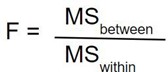
The test statistic for testing H 0 : μ 1 = μ 2 = ... = μ k is:
and the critical value is found in a table of probability values for the F distribution with (degrees of freedom) df 1 = k-1, df 2 =N-k. The table can be found in "Other Resources" on the left side of the pages.
NOTE: The test statistic F assumes equal variability in the k populations (i.e., the population variances are equal, or s 1 2 = s 2 2 = ... = s k 2 ). This means that the outcome is equally variable in each of the comparison populations. This assumption is the same as that assumed for appropriate use of the test statistic to test equality of two independent means. It is possible to assess the likelihood that the assumption of equal variances is true and the test can be conducted in most statistical computing packages. If the variability in the k comparison groups is not similar, then alternative techniques must be used.
The F statistic is computed by taking the ratio of what is called the "between treatment" variability to the "residual or error" variability. This is where the name of the procedure originates. In analysis of variance we are testing for a difference in means (H 0 : means are all equal versus H 1 : means are not all equal) by evaluating variability in the data. The numerator captures between treatment variability (i.e., differences among the sample means) and the denominator contains an estimate of the variability in the outcome. The test statistic is a measure that allows us to assess whether the differences among the sample means (numerator) are more than would be expected by chance if the null hypothesis is true. Recall in the two independent sample test, the test statistic was computed by taking the ratio of the difference in sample means (numerator) to the variability in the outcome (estimated by Sp).
The decision rule for the F test in ANOVA is set up in a similar way to decision rules we established for t tests. The decision rule again depends on the level of significance and the degrees of freedom. The F statistic has two degrees of freedom. These are denoted df 1 and df 2 , and called the numerator and denominator degrees of freedom, respectively. The degrees of freedom are defined as follows:
df 1 = k-1 and df 2 =N-k,
where k is the number of comparison groups and N is the total number of observations in the analysis. If the null hypothesis is true, the between treatment variation (numerator) will not exceed the residual or error variation (denominator) and the F statistic will small. If the null hypothesis is false, then the F statistic will be large. The rejection region for the F test is always in the upper (right-hand) tail of the distribution as shown below.
Rejection Region for F Test with a =0.05, df 1 =3 and df 2 =36 (k=4, N=40)

For the scenario depicted here, the decision rule is: Reject H 0 if F > 2.87.
The ANOVA Procedure
We will next illustrate the ANOVA procedure using the five step approach. Because the computation of the test statistic is involved, the computations are often organized in an ANOVA table. The ANOVA table breaks down the components of variation in the data into variation between treatments and error or residual variation. Statistical computing packages also produce ANOVA tables as part of their standard output for ANOVA, and the ANOVA table is set up as follows:
| Source of Variation | Sums of Squares (SS) | Degrees of Freedom (df) | Mean Squares (MS) | F |
|---|---|---|---|---|
| Between Treatments |
| k-1 |
|
|
| Error (or Residual) |
| N-k |
| |
| Total |
| N-1 |
where
- X = individual observation,
- k = the number of treatments or independent comparison groups, and
- N = total number of observations or total sample size.
The ANOVA table above is organized as follows.
- The first column is entitled "Source of Variation" and delineates the between treatment and error or residual variation. The total variation is the sum of the between treatment and error variation.
- The second column is entitled "Sums of Squares (SS)" . The between treatment sums of squares is
and is computed by summing the squared differences between each treatment (or group) mean and the overall mean. The squared differences are weighted by the sample sizes per group (n j ). The error sums of squares is:
and is computed by summing the squared differences between each observation and its group mean (i.e., the squared differences between each observation in group 1 and the group 1 mean, the squared differences between each observation in group 2 and the group 2 mean, and so on). The double summation ( SS ) indicates summation of the squared differences within each treatment and then summation of these totals across treatments to produce a single value. (This will be illustrated in the following examples). The total sums of squares is:
and is computed by summing the squared differences between each observation and the overall sample mean. In an ANOVA, data are organized by comparison or treatment groups. If all of the data were pooled into a single sample, SST would reflect the numerator of the sample variance computed on the pooled or total sample. SST does not figure into the F statistic directly. However, SST = SSB + SSE, thus if two sums of squares are known, the third can be computed from the other two.
- The third column contains degrees of freedom . The between treatment degrees of freedom is df 1 = k-1. The error degrees of freedom is df 2 = N - k. The total degrees of freedom is N-1 (and it is also true that (k-1) + (N-k) = N-1).
- The fourth column contains "Mean Squares (MS)" which are computed by dividing sums of squares (SS) by degrees of freedom (df), row by row. Specifically, MSB=SSB/(k-1) and MSE=SSE/(N-k). Dividing SST/(N-1) produces the variance of the total sample. The F statistic is in the rightmost column of the ANOVA table and is computed by taking the ratio of MSB/MSE.
A clinical trial is run to compare weight loss programs and participants are randomly assigned to one of the comparison programs and are counseled on the details of the assigned program. Participants follow the assigned program for 8 weeks. The outcome of interest is weight loss, defined as the difference in weight measured at the start of the study (baseline) and weight measured at the end of the study (8 weeks), measured in pounds.
Three popular weight loss programs are considered. The first is a low calorie diet. The second is a low fat diet and the third is a low carbohydrate diet. For comparison purposes, a fourth group is considered as a control group. Participants in the fourth group are told that they are participating in a study of healthy behaviors with weight loss only one component of interest. The control group is included here to assess the placebo effect (i.e., weight loss due to simply participating in the study). A total of twenty patients agree to participate in the study and are randomly assigned to one of the four diet groups. Weights are measured at baseline and patients are counseled on the proper implementation of the assigned diet (with the exception of the control group). After 8 weeks, each patient's weight is again measured and the difference in weights is computed by subtracting the 8 week weight from the baseline weight. Positive differences indicate weight losses and negative differences indicate weight gains. For interpretation purposes, we refer to the differences in weights as weight losses and the observed weight losses are shown below.
| Low Calorie | Low Fat | Low Carbohydrate | Control |
|---|---|---|---|
| 8 | 2 | 3 | 2 |
| 9 | 4 | 5 | 2 |
| 6 | 3 | 4 | -1 |
| 7 | 5 | 2 | 0 |
| 3 | 1 | 3 | 3 |
Is there a statistically significant difference in the mean weight loss among the four diets? We will run the ANOVA using the five-step approach.
- Step 1. Set up hypotheses and determine level of significance
H 0 : μ 1 = μ 2 = μ 3 = μ 4 H 1 : Means are not all equal α=0.05
- Step 2. Select the appropriate test statistic.
The test statistic is the F statistic for ANOVA, F=MSB/MSE.
- Step 3. Set up decision rule.
The appropriate critical value can be found in a table of probabilities for the F distribution(see "Other Resources"). In order to determine the critical value of F we need degrees of freedom, df 1 =k-1 and df 2 =N-k. In this example, df 1 =k-1=4-1=3 and df 2 =N-k=20-4=16. The critical value is 3.24 and the decision rule is as follows: Reject H 0 if F > 3.24.
- Step 4. Compute the test statistic.
To organize our computations we complete the ANOVA table. In order to compute the sums of squares we must first compute the sample means for each group and the overall mean based on the total sample.
|
| Low Calorie | Low Fat | Low Carbohydrate | Control |
|---|---|---|---|---|
| n | 5 | 5 | 5 | 5 |
| Group mean | 6.6 | 3.0 | 3.4 | 1.2 |
We can now compute
So, in this case:
Next we compute,
SSE requires computing the squared differences between each observation and its group mean. We will compute SSE in parts. For the participants in the low calorie diet:
|
| 6.6 |
|
|---|---|---|
| 8 | 1.4 | 2.0 |
| 9 | 2.4 | 5.8 |
| 6 | -0.6 | 0.4 |
| 7 | 0.4 | 0.2 |
| 3 | -3.6 | 13.0 |
| Totals | 0 | 21.4 |
For the participants in the low fat diet:
|
| 3.0 |
|
|---|---|---|
| 2 | -1.0 | 1.0 |
| 4 | 1.0 | 1.0 |
| 3 | 0.0 | 0.0 |
| 5 | 2.0 | 4.0 |
| 1 | -2.0 | 4.0 |
| Totals | 0 | 10.0 |
For the participants in the low carbohydrate diet:
|
|
|
|
|---|---|---|
| 3 | -0.4 | 0.2 |
| 5 | 1.6 | 2.6 |
| 4 | 0.6 | 0.4 |
| 2 | -1.4 | 2.0 |
| 3 | -0.4 | 0.2 |
| Totals | 0 | 5.4 |
For the participants in the control group:
|
|
|
|
|---|---|---|
| 2 | 0.8 | 0.6 |
| 2 | 0.8 | 0.6 |
| -1 | -2.2 | 4.8 |
| 0 | -1.2 | 1.4 |
| 3 | 1.8 | 3.2 |
| Totals | 0 | 10.6 |
We can now construct the ANOVA table .
| Source of Variation | Sums of Squares (SS) | Degrees of Freedom (df) | Means Squares (MS) | F |
|---|---|---|---|---|
| Between Treatmenst | 75.8 | 4-1=3 | 75.8/3=25.3 | 25.3/3.0=8.43 |
| Error (or Residual) | 47.4 | 20-4=16 | 47.4/16=3.0 | |
| Total | 123.2 | 20-1=19 |
- Step 5. Conclusion.
We reject H 0 because 8.43 > 3.24. We have statistically significant evidence at α=0.05 to show that there is a difference in mean weight loss among the four diets.
ANOVA is a test that provides a global assessment of a statistical difference in more than two independent means. In this example, we find that there is a statistically significant difference in mean weight loss among the four diets considered. In addition to reporting the results of the statistical test of hypothesis (i.e., that there is a statistically significant difference in mean weight losses at α=0.05), investigators should also report the observed sample means to facilitate interpretation of the results. In this example, participants in the low calorie diet lost an average of 6.6 pounds over 8 weeks, as compared to 3.0 and 3.4 pounds in the low fat and low carbohydrate groups, respectively. Participants in the control group lost an average of 1.2 pounds which could be called the placebo effect because these participants were not participating in an active arm of the trial specifically targeted for weight loss. Are the observed weight losses clinically meaningful?
Another ANOVA Example
Calcium is an essential mineral that regulates the heart, is important for blood clotting and for building healthy bones. The National Osteoporosis Foundation recommends a daily calcium intake of 1000-1200 mg/day for adult men and women. While calcium is contained in some foods, most adults do not get enough calcium in their diets and take supplements. Unfortunately some of the supplements have side effects such as gastric distress, making them difficult for some patients to take on a regular basis.
A study is designed to test whether there is a difference in mean daily calcium intake in adults with normal bone density, adults with osteopenia (a low bone density which may lead to osteoporosis) and adults with osteoporosis. Adults 60 years of age with normal bone density, osteopenia and osteoporosis are selected at random from hospital records and invited to participate in the study. Each participant's daily calcium intake is measured based on reported food intake and supplements. The data are shown below.
|
|
|
|
|---|---|---|
| 1200 | 1000 | 890 |
| 1000 | 1100 | 650 |
| 980 | 700 | 1100 |
| 900 | 800 | 900 |
| 750 | 500 | 400 |
| 800 | 700 | 350 |
Is there a statistically significant difference in mean calcium intake in patients with normal bone density as compared to patients with osteopenia and osteoporosis? We will run the ANOVA using the five-step approach.
H 0 : μ 1 = μ 2 = μ 3 H 1 : Means are not all equal α=0.05
In order to determine the critical value of F we need degrees of freedom, df 1 =k-1 and df 2 =N-k. In this example, df 1 =k-1=3-1=2 and df 2 =N-k=18-3=15. The critical value is 3.68 and the decision rule is as follows: Reject H 0 if F > 3.68.
To organize our computations we will complete the ANOVA table. In order to compute the sums of squares we must first compute the sample means for each group and the overall mean.
| Normal Bone Density |
|
|
|---|---|---|
| n =6 | n =6 | n =6 |
|
|
|
|
If we pool all N=18 observations, the overall mean is 817.8.
We can now compute:
Substituting:
SSE requires computing the squared differences between each observation and its group mean. We will compute SSE in parts. For the participants with normal bone density:
|
|
|
|
|---|---|---|
| 1200 | 261.6667 | 68,486.9 |
| 1000 | 61.6667 | 3,806.9 |
| 980 | 41.6667 | 1,738.9 |
| 900 | -38.3333 | 1,466.9 |
| 750 | -188.333 | 35,456.9 |
| 800 | -138.333 | 19,126.9 |
| Total | 0 | 130,083.3 |
For participants with osteopenia:
|
|
|
|
|---|---|---|
| 1000 | 200 | 40,000 |
| 1100 | 300 | 90,000 |
| 700 | -100 | 10,000 |
| 800 | 0 | 0 |
| 500 | -300 | 90,000 |
| 700 | -100 | 10,000 |
| Total | 0 | 240,000 |
For participants with osteoporosis:
|
|
|
|
|---|---|---|
| 890 | 175 | 30,625 |
| 650 | -65 | 4,225 |
| 1100 | 385 | 148,225 |
| 900 | 185 | 34,225 |
| 400 | -315 | 99,225 |
| 350 | -365 | 133,225 |
| Total | 0 | 449,750 |
|
|
|
|
|
|
|---|---|---|---|---|
| Between Treatments | 152,477.7 | 2 | 76,238.6 | 1.395 |
| Error or Residual | 819,833.3 | 15 | 54,655.5 | |
| Total | 972,311.0 | 17 |
We do not reject H 0 because 1.395 < 3.68. We do not have statistically significant evidence at a =0.05 to show that there is a difference in mean calcium intake in patients with normal bone density as compared to osteopenia and osterporosis. Are the differences in mean calcium intake clinically meaningful? If so, what might account for the lack of statistical significance?
One-Way ANOVA in R
The video below by Mike Marin demonstrates how to perform analysis of variance in R. It also covers some other statistical issues, but the initial part of the video will be useful to you.
Two-Factor ANOVA
The ANOVA tests described above are called one-factor ANOVAs. There is one treatment or grouping factor with k > 2 levels and we wish to compare the means across the different categories of this factor. The factor might represent different diets, different classifications of risk for disease (e.g., osteoporosis), different medical treatments, different age groups, or different racial/ethnic groups. There are situations where it may be of interest to compare means of a continuous outcome across two or more factors. For example, suppose a clinical trial is designed to compare five different treatments for joint pain in patients with osteoarthritis. Investigators might also hypothesize that there are differences in the outcome by sex. This is an example of a two-factor ANOVA where the factors are treatment (with 5 levels) and sex (with 2 levels). In the two-factor ANOVA, investigators can assess whether there are differences in means due to the treatment, by sex or whether there is a difference in outcomes by the combination or interaction of treatment and sex. Higher order ANOVAs are conducted in the same way as one-factor ANOVAs presented here and the computations are again organized in ANOVA tables with more rows to distinguish the different sources of variation (e.g., between treatments, between men and women). The following example illustrates the approach.
Consider the clinical trial outlined above in which three competing treatments for joint pain are compared in terms of their mean time to pain relief in patients with osteoarthritis. Because investigators hypothesize that there may be a difference in time to pain relief in men versus women, they randomly assign 15 participating men to one of the three competing treatments and randomly assign 15 participating women to one of the three competing treatments (i.e., stratified randomization). Participating men and women do not know to which treatment they are assigned. They are instructed to take the assigned medication when they experience joint pain and to record the time, in minutes, until the pain subsides. The data (times to pain relief) are shown below and are organized by the assigned treatment and sex of the participant.
Table of Time to Pain Relief by Treatment and Sex
|
|
|
|
|---|---|---|
|
| 12 | 21 |
| 15 | 19 | |
| 16 | 18 | |
| 17 | 24 | |
| 14 | 25 | |
|
| 14 | 21 |
| 17 | 20 | |
| 19 | 23 | |
| 20 | 27 | |
| 17 | 25 | |
|
| 25 | 37 |
| 27 | 34 | |
| 29 | 36 | |
| 24 | 26 | |
| 22 | 29 |
The analysis in two-factor ANOVA is similar to that illustrated above for one-factor ANOVA. The computations are again organized in an ANOVA table, but the total variation is partitioned into that due to the main effect of treatment, the main effect of sex and the interaction effect. The results of the analysis are shown below (and were generated with a statistical computing package - here we focus on interpretation).
ANOVA Table for Two-Factor ANOVA
|
|
|
|
|
|
|
|---|---|---|---|---|---|
| Model | 967.0 | 5 | 193.4 | 20.7 | 0.0001 |
| Treatment | 651.5 | 2 | 325.7 | 34.8 | 0.0001 |
| Sex | 313.6 | 1 | 313.6 | 33.5 | 0.0001 |
| Treatment * Sex | 1.9 | 2 | 0.9 | 0.1 | 0.9054 |
| Error or Residual | 224.4 | 24 | 9.4 | ||
| Total | 1191.4 | 29 |
There are 4 statistical tests in the ANOVA table above. The first test is an overall test to assess whether there is a difference among the 6 cell means (cells are defined by treatment and sex). The F statistic is 20.7 and is highly statistically significant with p=0.0001. When the overall test is significant, focus then turns to the factors that may be driving the significance (in this example, treatment, sex or the interaction between the two). The next three statistical tests assess the significance of the main effect of treatment, the main effect of sex and the interaction effect. In this example, there is a highly significant main effect of treatment (p=0.0001) and a highly significant main effect of sex (p=0.0001). The interaction between the two does not reach statistical significance (p=0.91). The table below contains the mean times to pain relief in each of the treatments for men and women (Note that each sample mean is computed on the 5 observations measured under that experimental condition).
Mean Time to Pain Relief by Treatment and Gender
|
|
|
|
|---|---|---|
| A | 14.8 | 21.4 |
| B | 17.4 | 23.2 |
| C | 25.4 | 32.4 |
Treatment A appears to be the most efficacious treatment for both men and women. The mean times to relief are lower in Treatment A for both men and women and highest in Treatment C for both men and women. Across all treatments, women report longer times to pain relief (See below).

Notice that there is the same pattern of time to pain relief across treatments in both men and women (treatment effect). There is also a sex effect - specifically, time to pain relief is longer in women in every treatment.
Suppose that the same clinical trial is replicated in a second clinical site and the following data are observed.
Table - Time to Pain Relief by Treatment and Sex - Clinical Site 2
|
|
|
|
|---|---|---|
|
| 22 | 21 |
| 25 | 19 | |
| 26 | 18 | |
| 27 | 24 | |
| 24 | 25 | |
|
| 14 | 21 |
| 17 | 20 | |
| 19 | 23 | |
| 20 | 27 | |
| 17 | 25 | |
|
| 15 | 37 |
| 17 | 34 | |
| 19 | 36 | |
| 14 | 26 | |
| 12 | 29 |
The ANOVA table for the data measured in clinical site 2 is shown below.
Table - Summary of Two-Factor ANOVA - Clinical Site 2
| Source of Variation | Sums of Squares (SS) | Degrees of freedom (df) | Mean Squares (MS) | F | P-Value |
|---|---|---|---|---|---|
| Model | 907.0 | 5 | 181.4 | 19.4 | 0.0001 |
| Treatment | 71.5 | 2 | 35.7 | 3.8 | 0.0362 |
| Sex | 313.6 | 1 | 313.6 | 33.5 | 0.0001 |
| Treatment * Sex | 521.9 | 2 | 260.9 | 27.9 | 0.0001 |
| Error or Residual | 224.4 | 24 | 9.4 | ||
| Total | 1131.4 | 29 |
Notice that the overall test is significant (F=19.4, p=0.0001), there is a significant treatment effect, sex effect and a highly significant interaction effect. The table below contains the mean times to relief in each of the treatments for men and women.
Table - Mean Time to Pain Relief by Treatment and Gender - Clinical Site 2
|
|
|
|
|---|---|---|
|
| 24.8 | 21.4 |
|
| 17.4 | 23.2 |
|
| 15.4 | 32.4 |
Notice that now the differences in mean time to pain relief among the treatments depend on sex. Among men, the mean time to pain relief is highest in Treatment A and lowest in Treatment C. Among women, the reverse is true. This is an interaction effect (see below).

Notice above that the treatment effect varies depending on sex. Thus, we cannot summarize an overall treatment effect (in men, treatment C is best, in women, treatment A is best).
When interaction effects are present, some investigators do not examine main effects (i.e., do not test for treatment effect because the effect of treatment depends on sex). This issue is complex and is discussed in more detail in a later module.
ANOVA Test: Definition, Types, Examples, SPSS
Statistics Definitions > ANOVA Contents :
The ANOVA Test
- How to Run a One Way ANOVA in SPSS
Two Way ANOVA
What is manova, what is factorial anova, how to run an anova, anova vs. t test.
- Repeated Measures ANOVA in SPSS: Steps
Related Articles
Watch the video for an introduction to ANOVA.

Can’t see the video? Click here to watch it on YouTube.
An ANOVA test is a way to find out if survey or experiment results are significant . In other words, they help you to figure out if you need to reject the null hypothesis or accept the alternate hypothesis .
Basically, you’re testing groups to see if there’s a difference between them. Examples of when you might want to test different groups:
- A group of psychiatric patients are trying three different therapies: counseling, medication and biofeedback. You want to see if one therapy is better than the others.
- A manufacturer has two different processes to make light bulbs. They want to know if one process is better than the other.
- Students from different colleges take the same exam. You want to see if one college outperforms the other.
What Does “One-Way” or “Two-Way Mean?
One-way or two-way refers to the number of independent variables (IVs) in your Analysis of Variance test.
- One-way has one independent variable (with 2 levels ). For example: brand of cereal ,
- Two-way has two independent variables (it can have multiple levels). For example: brand of cereal, calories .
What are “Groups” or “Levels”?
Groups or levels are different groups within the same independent variable . In the above example, your levels for “brand of cereal” might be Lucky Charms, Raisin Bran, Cornflakes — a total of three levels. Your levels for “Calories” might be: sweetened, unsweetened — a total of two levels.
Let’s say you are studying if an alcoholic support group and individual counseling combined is the most effective treatment for lowering alcohol consumption. You might split the study participants into three groups or levels:
- Medication only,
- Medication and counseling,
- Counseling only.
Your dependent variable would be the number of alcoholic beverages consumed per day.
If your groups or levels have a hierarchical structure (each level has unique subgroups), then use a nested ANOVA for the analysis.
What Does “Replication” Mean?
It’s whether you are replicating (i.e. duplicating) your test(s) with multiple groups. With a two way ANOVA with replication , you have two groups and individuals within that group are doing more than one thing (i.e. two groups of students from two colleges taking two tests). If you only have one group taking two tests, you would use without replication.
Types of Tests.
There are two main types: one-way and two-way. Two-way tests can be with or without replication.
- One-way ANOVA between groups: used when you want to test two groups to see if there’s a difference between them.
- Two way ANOVA without replication: used when you have one group and you’re double-testing that same group. For example, you’re testing one set of individuals before and after they take a medication to see if it works or not.
- Two way ANOVA with replication: Two groups , and the members of those groups are doing more than one thing . For example, two groups of patients from different hospitals trying two different therapies.
Back to Top
One Way ANOVA
A one way ANOVA is used to compare two means from two independent (unrelated) groups using the F-distribution . The null hypothesis for the test is that the two means are equal. Therefore, a significant result means that the two means are unequal.
Examples of when to use a one way ANOVA
Situation 1: You have a group of individuals randomly split into smaller groups and completing different tasks. For example, you might be studying the effects of tea on weight loss and form three groups: green tea, black tea, and no tea. Situation 2: Similar to situation 1, but in this case the individuals are split into groups based on an attribute they possess. For example, you might be studying leg strength of people according to weight. You could split participants into weight categories (obese, overweight and normal) and measure their leg strength on a weight machine.
Limitations of the One Way ANOVA
A one way ANOVA will tell you that at least two groups were different from each other. But it won’t tell you which groups were different. If your test returns a significant f-statistic, you may need to run an ad hoc test (like the Least Significant Difference test) to tell you exactly which groups had a difference in means . Back to Top
How to run a One Way ANOVA in SPSS
A Two Way ANOVA is an extension of the One Way ANOVA. With a One Way, you have one independent variable affecting a dependent variable . With a Two Way ANOVA, there are two independents. Use a two way ANOVA when you have one measurement variable (i.e. a quantitative variable ) and two nominal variables . In other words, if your experiment has a quantitative outcome and you have two categorical explanatory variables , a two way ANOVA is appropriate.
For example, you might want to find out if there is an interaction between income and gender for anxiety level at job interviews. The anxiety level is the outcome, or the variable that can be measured. Gender and Income are the two categorical variables . These categorical variables are also the independent variables, which are called factors in a Two Way ANOVA.
The factors can be split into levels . In the above example, income level could be split into three levels: low, middle and high income. Gender could be split into three levels: male, female, and transgender. Treatment groups are all possible combinations of the factors. In this example there would be 3 x 3 = 9 treatment groups.
Main Effect and Interaction Effect
The results from a Two Way ANOVA will calculate a main effect and an interaction effect . The main effect is similar to a One Way ANOVA: each factor’s effect is considered separately. With the interaction effect, all factors are considered at the same time. Interaction effects between factors are easier to test if there is more than one observation in each cell. For the above example, multiple stress scores could be entered into cells. If you do enter multiple observations into cells, the number in each cell must be equal.
Two null hypotheses are tested if you are placing one observation in each cell. For this example, those hypotheses would be: H 01 : All the income groups have equal mean stress. H 02 : All the gender groups have equal mean stress.
For multiple observations in cells, you would also be testing a third hypothesis: H 03 : The factors are independent or the interaction effect does not exist.
An F-statistic is computed for each hypothesis you are testing.
Assumptions for Two Way ANOVA
- The population must be close to a normal distribution .
- Samples must be independent.
- Population variances must be equal (i.e. homoscedastic ).
- Groups must have equal sample sizes .
MANOVA is just an ANOVA with several dependent variables. It’s similar to many other tests and experiments in that it’s purpose is to find out if the response variable (i.e. your dependent variable) is changed by manipulating the independent variable. The test helps to answer many research questions, including:
- Do changes to the independent variables have statistically significant effects on dependent variables?
- What are the interactions among dependent variables?
- What are the interactions among independent variables?
MANOVA Example
Suppose you wanted to find out if a difference in textbooks affected students’ scores in math and science. Improvements in math and science means that there are two dependent variables, so a MANOVA is appropriate.
An ANOVA will give you a single ( univariate ) f-value while a MANOVA will give you a multivariate F value. MANOVA tests the multiple dependent variables by creating new, artificial, dependent variables that maximize group differences. These new dependent variables are linear combinations of the measured dependent variables.
Interpreting the MANOVA results
If the multivariate F value indicates the test is statistically significant , this means that something is significant. In the above example, you would not know if math scores have improved, science scores have improved (or both). Once you have a significant result, you would then have to look at each individual component (the univariate F tests) to see which dependent variable(s) contributed to the statistically significant result.
Advantages and Disadvantages of MANOVA vs. ANOVA
- MANOVA enables you to test multiple dependent variables.
- MANOVA can protect against Type I errors.
Disadvantages
- MANOVA is many times more complicated than ANOVA, making it a challenge to see which independent variables are affecting dependent variables.
- One degree of freedom is lost with the addition of each new variable .
- The dependent variables should be uncorrelated as much as possible. If they are correlated, the loss in degrees of freedom means that there isn’t much advantages in including more than one dependent variable on the test.
Reference : SFSU. Retrieved April 18, 2022 from: http://online.sfsu.edu/efc/classes/biol710/manova/MANOVAnewest.pdf
A factorial ANOVA is an Analysis of Variance test with more than one independent variable , or “ factor “. It can also refer to more than one Level of Independent Variable . For example, an experiment with a treatment group and a control group has one factor (the treatment) but two levels (the treatment and the control). The terms “two-way” and “three-way” refer to the number of factors or the number of levels in your test. Four-way ANOVA and above are rarely used because the results of the test are complex and difficult to interpret.
- A two-way ANOVA has two factors ( independent variables ) and one dependent variable . For example, time spent studying and prior knowledge are factors that affect how well you do on a test.
- A three-way ANOVA has three factors (independent variables) and one dependent variable. For example, time spent studying, prior knowledge, and hours of sleep are factors that affect how well you do on a test
Factorial ANOVA is an efficient way of conducting a test. Instead of performing a series of experiments where you test one independent variable against one dependent variable, you can test all independent variables at the same time.
Variability
In a one-way ANOVA, variability is due to the differences between groups and the differences within groups. In factorial ANOVA, each level and factor are paired up with each other (“crossed”). This helps you to see what interactions are going on between the levels and factors. If there is an interaction then the differences in one factor depend on the differences in another.
Let’s say you were running a two-way ANOVA to test male/female performance on a final exam. The subjects had either had 4, 6, or 8 hours of sleep.
- IV1: SEX (Male/Female)
- IV2: SLEEP (4/6/8)
- DV: Final Exam Score
A two-way factorial ANOVA would help you answer the following questions:
- Is sex a main effect? In other words, do men and women differ significantly on their exam performance?
- Is sleep a main effect? In other words, do people who have had 4,6, or 8 hours of sleep differ significantly in their performance?
- Is there a significant interaction between factors? In other words, how do hours of sleep and sex interact with regards to exam performance?
- Can any differences in sex and exam performance be found in the different levels of sleep?
Assumptions of Factorial ANOVA
- Normality: the dependent variable is normally distributed.
- Independence: Observations and groups are independent from each other.
- Equality of Variance: the population variances are equal across factors/levels.
These tests are very time-consuming by hand. In nearly every case you’ll want to use software. For example, several options are available in Excel :
- Two way ANOVA in Excel with replication and without replication.
- One way ANOVA in Excel 2013 .

ANOVA tests in statistics packages are run on parametric data. If you have rank or ordered data, you’ll want to run a non-parametric ANOVA (usually found under a different heading in the software, like “ nonparametric tests “).
It is unlikely you’ll want to do this test by hand, but if you must, these are the steps you’ll want to take:
- Find the mean for each of the groups.
- Find the overall mean (the mean of the groups combined).
- Find the Within Group Variation ; the total deviation of each member’s score from the Group Mean.
- Find the Between Group Variation : the deviation of each Group Mean from the Overall Mean.
- Find the F statistic: the ratio of Between Group Variation to Within Group Variation.
A Student’s t-test will tell you if there is a significant variation between groups. A t-test compares means, while the ANOVA compares variances between populations. You could technically perform a series of t-tests on your data. However, as the groups grow in number, you may end up with a lot of pair comparisons that you need to run. ANOVA will give you a single number (the f-statistic ) and one p-value to help you support or reject the null hypothesis . Back to Top
Repeated Measures (Within Subjects) ANOVA
A repeated measures ANOVA is almost the same as one-way ANOVA, with one main difference: you test related groups, not independent ones.
It’s called Repeated Measures because the same group of participants is being measured over and over again. For example, you could be studying the cholesterol levels of the same group of patients at 1, 3, and 6 months after changing their diet. For this example, the independent variable is “time” and the dependent variable is “cholesterol.” The independent variable is usually called the within-subjects factor .
Repeated measures ANOVA is similar to a simple multivariate design. In both tests, the same participants are measured over and over. However, with repeated measures the same characteristic is measured with a different condition. For example, blood pressure is measured over the condition “time”. For simple multivariate design it is the characteristic that changes. For example, you could measure blood pressure, heart rate and respiration rate over time.
Reasons to use Repeated Measures ANOVA
- When you collect data from the same participants over a period of time, individual differences (a source of between group differences) are reduced or eliminated.
- Testing is more powerful because the sample size isn’t divided between groups.
- The test can be economical, as you’re using the same participants.
Assumptions for Repeated Measures ANOVA
The results from your repeated measures ANOVA will be valid only if the following assumptions haven’t been violated:
- There must be one independent variable and one dependent variable.
- The dependent variable must be a continuous variable , on an interval scale or a ratio scale .
- The independent variable must be categorical , either on the nominal scale or ordinal scale.
- Ideally, levels of dependence between pairs of groups is equal (“sphericity”). Corrections are possible if this assumption is violated.
One Way Repeated Measures ANOVA in SPSS: Steps
Watch the video for the steps:

Step 2: Replace the “factor1” name with something that represents your independent variable. For example, you could put “age” or “time.”
Step 3: Enter the “Number of Levels.” This is how many times the dependent variable has been measured. For example, if you took measurements every week for a total of 4 weeks, this number would be 4.
Step 4: Click the “Add” button and then give your dependent variable a name.

Step 7: Click “Plots” and use the arrow keys to transfer the factor from the left box onto the Horizontal Axis box.

Step 9: Click “Options”, then transfer your factors from the left box to the Display Means for box on the right.
Step 10: Click the following check boxes:
- Compare main effects.
- Descriptive Statistics.
- Estimates of Effect Size .
Step 11: Select “Bonferroni” from the drop down menu under Confidence Interval Adjustment . Step 12: Click “Continue” and then click “OK” to run the test. Back to Top
In statistics, sphericity (ε) refers to Mauchly’s sphericity test , which was developed in 1940 by John W. Mauchly , who co-developed the first general-purpose electronic computer.
Sphericity is used as an assumption in repeated measures ANOVA. The assumption states that the variances of the differences between all possible group pairs are equal. If your data violates this assumption, it can result in an increase in a Type I error (the incorrect rejection of the null hypothesis) .
It’s very common for repeated measures ANOVA to result in a violation of the assumption. If the assumption has been violated, corrections have been developed that can avoid increases in the type I error rate. The correction is applied to the degrees of freedom in the F-distribution .
Mauchly’s Sphericity Test
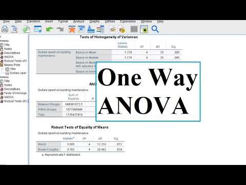
Mauchly’s test for sphericity can be run in the majority of statistical software, where it tends to be the default test for sphericity. Mauchly’s test is ideal for mid-size samples. It may fail to detect sphericity in small samples and it may over-detect in large samples. If the test returns a small p-value (p ≤.05), this is an indication that your data has violated the assumption. The following picture of SPSS output for ANOVA shows that the significance “sig” attached to Mauchly’s is .274. This means that the assumption has not been violated for this set of data.
You would report the above result as “Mauchly’s Test indicated that the assumption of sphericity had not been violated, χ 2 (2) = 2.588, p = .274.”
If your test returned a small p-value , you should apply a correction, usually either the:
- Greehouse-Geisser correction.
- Huynh-Feldt correction .
When ε ≤ 0.75 (or you don’t know what the value for the statistic is), use the Greenhouse-Geisser correction. When ε > .75, use the Huynh-Feldt correction .
Grand mean ANOVA vs Regression
Blokdyk, B. (2018). Ad Hoc Testing . 5STARCooks Miller, R. G. Beyond ANOVA: Basics of Applied Statistics . Boca Raton, FL: Chapman & Hall, 1997 Image: UVM. Retrieved December 4, 2020 from: https://www.uvm.edu/~dhowell/gradstat/psych341/lectures/RepeatedMeasures/repeated1.html
Hypothesis tests about the variance
by Marco Taboga , PhD
This page explains how to perform hypothesis tests about the variance of a normal distribution, called Chi-square tests.
We analyze two different situations:
when the mean of the distribution is known;
when it is unknown.
Depending on the situation, the Chi-square statistic used in the test has a different distribution.
At the end of the page, we propose some solved exercises.
Table of contents
Normal distribution with known mean
The null hypothesis, the test statistic, the critical region, the decision, the power function, the size of the test, how to choose the critical value, normal distribution with unknown mean, solved exercises.
The assumptions are the same previously made in the lecture on confidence intervals for the variance .
The sample is drawn from a normal distribution .
A test of hypothesis based on it is called a Chi-square test .
Otherwise the null is not rejected.
![[eq8]](https://www.statlect.com/images/hypothesis-testing-variance__21.png "example of variability hypothesis")
We explain how to do this in the page on critical values .
We now relax the assumption that the mean of the distribution is known.
![[eq29]](https://www.statlect.com/images/hypothesis-testing-variance__74.png "example of variability hypothesis")
See the comments on the choice of the critical value made for the case of known mean.
Below you can find some exercises with explained solutions.
Suppose that we observe 40 independent realizations of a normal random variable.
we run a Chi-square test of the null hypothesis that the variance is equal to 1;
Make the same assumptions of Exercise 1 above.
If the unadjusted sample variance is equal to 0.9, is the null hypothesis rejected?
How to cite
Please cite as:
Taboga, Marco (2021). "Hypothesis tests about the variance", Lectures on probability theory and mathematical statistics. Kindle Direct Publishing. Online appendix. https://www.statlect.com/fundamentals-of-statistics/hypothesis-testing-variance.
Most of the learning materials found on this website are now available in a traditional textbook format.
- Convergence in probability
- Multivariate normal distribution
- Characteristic function
- Moment generating function
- Chi-square distribution
- Beta function
- Bernoulli distribution
- Mathematical tools
- Fundamentals of probability
- Probability distributions
- Asymptotic theory
- Fundamentals of statistics
- About Statlect
- Cookies, privacy and terms of use
- Posterior probability
- IID sequence
- Probability space
- Probability density function
- Continuous mapping theorem
- To enhance your privacy,
- we removed the social buttons,
- but don't forget to share .

14 Chapter 14: Analysis of Variance
Additional hypothesis tests.
In unit 1, we learned the basics of statistics – what they are, how they work, and the mathematical and conceptual principles that guide them. In unit 2, we put applied these principles to the process and ideas of hypothesis testing – how we take observed sample data and use it to make inferences about our populations of interest – using one continuous variable and one categorical variable. We will now continue to use this same hypothesis testing logic and procedure on new types of data. We will focus on group mean differences on more than two groups, using Analysis of Variance.
Analysis of variance, often abbreviated to ANOVA for short, serves the same purpose as the t -tests we learned earlier in unit 2: it tests for differences in group means. ANOVA is more flexible in that it can handle any number of groups, unlike t -tests which are limited to two groups (independent samples) or two time points (paired samples). Thus, the purpose and interpretation of ANOVA will be the same as it was for t -tests, as will the hypothesis testing procedure. However, ANOVA will, at first glance, look much different from a mathematical perspective, though as we will see, the basic logic behind the test statistic for ANOVA is actually the same.
ANOVA basics
An Analysis of Variance (ANOVA) is an inferential statistical tool that we use to find statistically significant differences among the means of two or more populations.
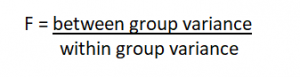
We calculate variance but the goal is still to compare population mean differences. The test statistic for the ANOVA is called F. It is a ratio of two estimates of the population variance based on the sample data.
Experiments are designed to determine if there is a cause and effect relationship between two variables. In the language of the ANOVA, the factor is the variable hypothesized to cause some change (effect) in the response variable (dependent variable).
An ANOVA conducted on a design in which there is only one factor is called a one-way ANOVA . If an experiment has two factors, then the ANOVA is called a two-way ANOVA . For example, suppose an experiment on the effects of age and gender on reading speed were conducted using three age groups (8 years, 10 years, and 12 years) and the two genders (male and female). The factors would be age and gender. Age would have three levels and gender would have two levels. ANOVAs can also be used for within-group/repeated and between subjects designs. For this chapter we will focus on between subject one-way ANOVA .
In a One-Way ANOVA we compare two types of variance: the variance between groups and the variance within groups, which we will discuss in the next section.
Observing and Interpreting Variability
We have seen time and again that scores, be they individual data or group means, will differ naturally. Sometimes this is due to random chance, and other times it is due to actual differences. Our job as scientists, researchers, and data analysts is to determine if the observed differences are systematic and meaningful (via a hypothesis test) and, if so, what is causing those differences. Through this, it becomes clear that, although we are usually interested in the mean or average score, it is the variability in the scores that is key.
Take a look at figure 1, which shows scores for many people on a test of skill used as part of a job application. The x-axis has each individual person, in no particular order, and the y-axis contains the score each person received on the test. As we can see, the job applicants differed quite a bit in their performance, and understanding why that is the case would be extremely useful information. However, there’s no interpretable pattern in the data, especially because we only have information on the test, not on any other variable (remember that the x-axis here only shows individual people and is not ordered or interpretable).

Figure 1. Scores on a job test
Our goal is to explain this variability that we are seeing in the dataset. Let’s assume that as part of the job application procedure we also collected data on the highest degree each applicant earned. With knowledge of what the job requires, we could sort our applicants into three groups: those applicants who have a college degree related to the job, those applicants who have a college degree that is not related to the job, and those applicants who did not earn a college degree. This is a common way that job applicants are sorted, and we can use ANOVA to test if these groups are actually different. Figure 2 presents the same job applicant scores, but now they are color coded by group membership (i.e. which group they belong in). Now that we can differentiate between applicants this way, a pattern starts to emerge: those applicants with a relevant degree (coded red) tend to be near the top, those applicants with no college degree (coded black) tend to be near the bottom, and the applicants with an unrelated degree (coded green) tend to fall into the middle. However, even within these groups, there is still some variability, as shown in Figure 2.

Figure 2. Applicant scores coded by degree earned
This pattern is even easier to see when the applicants are sorted and organized into their respective groups, as shown in Figure 3.

Figure 3. Applicant scores by group
Now that we have our data visualized into an easily interpretable format, we can clearly see that our applicants’ scores differ largely along group lines. Those applicants who do not have a college degree received the lowest scores, those who had a degree relevant to the job received the highest scores, and those who did have a degree but one that is not related to the job tended to fall somewhere in the middle. Thus, we have systematic variance between our groups.
The process and analyses used in ANOVA will take these two sources of variance (systematic variance between groups and random error within groups, or how much groups differ from each other and how much people differ within each group) and compare them to one another to determine if the groups have any explanatory value in our outcome variable. By doing this, we will test for statistically significant differences between the group means, just like we did for t – tests. We will go step by step to break down the math to see how ANOVA actually works.
Sources of Variance
ANOVA is all about looking at the different sources of variance (i.e. the reasons that scores differ from one another) in a dataset. Fortunately, the way we calculate these sources of variance takes a very familiar form: the Sum of Squares. Before we get into the calculations themselves, we must first lay out some important terminology and notation.
In ANOVA, we are working with two variables, a grouping or explanatory variable and a continuous outcome variable . The grouping variable is our predictor (it predicts or explains the values in the outcome variable) or, in experimental terms, our independent variable , and it made up of k groups, with k being any whole number 2 or greater. That is, ANOVA requires two or more groups to work, and it is usually conducted with three or more. In ANOVA, we refer to groups as “levels”, so the number of levels is just the number of groups, which again is k . In the above example, our grouping variable was education, which had 3 levels, so k = 3. When we report any descriptive value (e.g. mean, sample size, standard deviation) for a specific group, we will use a subscript 1… k to denote which group it refers to. For example, if we have three groups and want to report the standard deviation s for each group, we would report them as s 1 , s 2 , and s 3 .
Our second variable is our outcome variable . This is the variable on which people differ, and we are trying to explain or account for those differences based on group membership. In the example above, our outcome was the score each person earned on the test. Our outcome variable will still use X for scores as before. When describing the outcome variable using means, we will use subscripts to refer to specific group means. So if we have k = 3 groups, our means will be ̅X̅1̅, ̅X̅2̅, and ̅X̅3̅. We will also have a single mean representing the average of all participants across all groups. This is known as the grand mean , and we use the symbol X̅G. These different means – the individual group means and the overall grand mean –will be how we calculate our sums of squares.
Finally, we now have to differentiate between several different sample sizes. Our data will now have sample sizes for each group, and we will denote these with a lower case “n” and a subscript, just like with our other descriptive statistics: n 1 , n 2 , and n 3 . We also have the overall sample size in our dataset, and we will denote this with a capital N. The total sample size (N) is just the group sample sizes added together.
Between Groups Sum of Squares
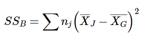
One source of variability we can identified in Figure 3 of the above example was differences or variability between the groups. That is, the groups clearly had different average levels. The variability arising from these differences is known as the between groups variability, and it is quantified using Between Groups Sum of Squares.
Our calculations for sums of squares in ANOVA will take on the same form as it did for regular calculations of variance. Each observation, in this case the group means, is compared to the overall mean, in this case the grand mean, to calculate a deviation score. These deviation scores are squared so that they do not cancel each other out and sum to zero. The squared deviations are then added up, or summed. There is, however, one small difference. Because each group mean represents a group composed of multiple people, before we sum the deviation scores we must multiple them by the number of people within that group. Incorporating this, we find our equation for Between Groups Sum of Squares.
Within Groups Sum of Squares
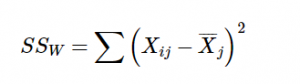
The other source of variability in the figures comes from differences that occur within each group. That is, each individual deviates a little bit from their respective group mean, just like the group means differed from the grand mean. We therefore label this source the Within Groups Sum of Squares. Because we are trying to account for variance based on group-level means, any deviation from the group means indicates an inaccuracy or error. Thus, our within groups variability represents our error in ANOVA.
We can see that our Total Sum of Squares is just each individual score minus the grand mean. As with our Within Groups Sum of Squares, we are calculating a deviation score for each individual person, so we do not need to multiply anything by the sample size; that is only done for Between Groups Sum of Squares.

This will prove to be very convenient, because if we know the values of any two of our sums of squares, it is very quick and easy to find the value of the third. It is also a good way to check calculations: if you calculate each SS by hand, you can make sure that they all fit together as shown above, and if not, you know that you made a math mistake somewhere.
We can see from the above formulas that calculating an ANOVA by hand from raw data can take a very, very long time. For this reason, you will not be required to calculate the SS values by hand, but you should still take the time to understand how they fit together and what each one represents to ensure you understand the analysis itself.
ANOVA Table
All of our sources of variability fit together in meaningful, interpretable ways as we saw above, and the easiest way to do this is to organize them into a table. The ANOVA table, shown in Table 1, is how we calculate our test statistic.
| Source | SS | df | MS | F |
| Between | SS | k-1 |
|
|
| Within | SS | N-k |
|
|
| Total | SS | N-1 | (MS is variance) |
|
Table 1. ANOVA table.
The first column of the ANOVA table, labeled “Source”, indicates which of our sources of variability we are using: between groups, within groups, or total. The second column, labeled “SS”, contains our values for the sums of squares that we learned to calculate above. As noted previously, calculating these by hand takes too long, and so the formulas are not presented in Table 1. However, remember that the Total is the sum of the other two, in case you are only given two SS values and need to calculate the third.
The next column in Table 1, labeled “df”, is our degrees of freedom. As with the sums of squares, there is a different df for each group, and the formulas are presented in the table. Notice that the total degrees of freedom, N – 1, is the same as it was for our regular variance. This matches the SS T formulation to again indicate that we are simply taking our familiar variance term and breaking it up into difference sources. Also remember that the capital N in the df calculations refers to the overall sample size, not a specific group sample size. Notice that the total row for degrees of freedom, just like for sums of squares, is just the Between and Within rows added together. If you take N – k + k – 1, then the “– k” and “+ k” portions will cancel out, and you are left with N – 1. This is a convenient way to quickly check your calculations.
The third column, labeled “MS”, is our Mean Squares for each source of variance. A “mean square” is just another way to say variability. Each mean square is calculated by dividing the sum of squares by its corresponding degrees of freedom. Notice that we do this for the Between row and the Within row, but not for the Total row. There are two reasons for this. First, our Total Mean Square would just be the variance in the full dataset (put together the formulas to see this for yourself), so it would not be new information. Second, the Mean Square values for Between and Within would not add up to equal the Mean Square Total because they are divided by different denominators. This is in contrast to the first two columns, where the Total row was both the conceptual total (i.e. the overall variance and degrees of freedom) and the literal total of the other two rows.
The final column in the ANOVA table (Table 1), labeled “F”, is our test statistic for ANOVA. The F statistic, just like a t – or z -statistic, is compared to a critical value to see whether we can reject for fail to reject a null hypothesis. Thus, although the calculations look different for ANOVA, we are still doing the same thing that we did in all of Unit 2. We are simply using a new type of data to test our hypotheses. We will see what these hypotheses look like shortly, but first, we must take a moment to address why we are doing our calculations this way.
We will typically work from having Sum of Squares calculated, but here are the basic formulas for the 3 types of Sum of Squares for the ANOVA:
- Total sum of squares (SS T ): ∑ x 2 – (∑x)2/n
- Within sum of squares (SS W ): add up the sum of squares for each treatment condition
- Between sum of squares (SS B ): SST – SSW = SSB
While there are other ways to calculate the SSs, these are the formulas we can use for this class if needed.
ANOVA and Type I Error
You may be wondering why we do not just use another t -test to test our hypotheses about three or more groups the way we did in Unit 2. After all, we are still just looking at group mean differences. The reason is that our t -statistic formula can only handle up to two groups, one minus the other. With only two groups, we can move our population parameters for the group means around in our null hypothesis and still get the same interpretation: the means are equal, which can also be concluded if one mean minus the other mean is equal to zero. However, if we tried adding a third mean, we would no longer be able to do this. So, in order to use t – tests to compare three or more means, we would have to run a series of individual group comparisons.
For only three groups, we would have three t -tests: group 1 vs group 2, group 1 vs group 3, and group 2 vs group 3. This may not sound like a lot, especially with the advances in technology that have made running an analysis very fast, but it quickly scales up. With just one additional group, bringing our total to four, we would have six comparisons: group 1 vs group 2, group 1 vs group 3, group 1 vs group 4, group 2 vs group 3, group 2 vs group 4, and group 3 vs group 4. This makes for a logistical and computation nightmare for five or more groups. When we reject the null hypothesis in a one-way ANOVA, we conclude that the group means are not all the same in the population. But this can indicate different things. With three groups, it can indicate that all three means are significantly different from each other. Or it can indicate that one of the means is significantly different from the other two, but the other two are not significantly different from each other. For this reason, statistically significant one-way ANOVA results are typically followed up with a series of post hoc comparisons of selected pairs of group means to determine which are different from which others.
A bigger issue, however, is our probability of committing a Type I Error. Remember that a Type I error is a false positive, and the chance of committing a Type I error is equal to our significance level, α. This is true if we are only running a single analysis (such as a t -test with only two groups) on a single dataset.
However, when we start running multiple analyses on the same dataset, our Type I error rate increases, raising the probability that we are capitalizing on random chance and rejecting a null hypothesis when we should not. ANOVA, by comparing all groups simultaneously with a single analysis, averts this issue and keeps our error rate at the α we set.
Hypotheses in ANOVA
So far we have seen what ANOVA is used for, why we use it, and how we use it. Now we can turn to the formal hypotheses we will be testing. As with before, we have a null and an alternative hypothesis to lay out. Our null hypothesis is still the idea of “no difference” in our data. Because we have multiple group means, we simply list them out as equal to each other:
H 0 : There is no difference in the group means. H0: µ1 = µ2 = µ3
We list as many μ parameters as groups we have. In the example above, we have three groups to test (k = 3), so we have three parameters in our null hypothesis. If we had more groups, say, four, we would simply add another μ to the list and give it the appropriate subscript, giving us: H0: µ1 = µ2 = µ3 = µ4. Notice that we do not say that the means are all equal to zero, we only say that they are equal to one another; it does not matter what the actual value is, so long as it holds for all groups equally.
Our alternative hypothesis for ANOVA is a little bit different. Let’s take a look at it and then dive deeper into what it means:
H A : At least 1 mean is different
The first difference in obvious: there is no mathematical statement of the alternative hypothesis in ANOVA. This is due to the second difference: we are not saying which group is going to be different, only that at least one will be. Because we do not hypothesize about which mean will be different, there is no way to write it mathematically. Related to this, we do not have directional hypotheses (greater than or less than) like we did with the z-statistic and t- statistics. Due to this, our alternative hypothesis is always exactly the same: at least one mean is different.
With t-tests, we saw that, if we reject the null hypothesis, we can adopt the alternative, and this made it easy to understand what the differences looked like. In ANOVA, we will still adopt the alternative hypothesis as the best explanation of our data if we reject the null hypothesis. However, when we look at the alternative hypothesis, we can see that it does not give us much information. We will know that a difference exists somewhere, but we will not know where that difference is. The ANOVA is an ominous test meaning you just know there are differences. More specifically, at least 1 group is different from the rest. Is only group 1 different but groups 2 and 3 the same? Is it only group 2? Are all three of them different? Based on just our alternative hypothesis, there is no way to be sure. We will come back to this issue later and see how to find out specific differences. For now, just remember that we are testing for any difference in group means, and it does not matter where that difference occurs. Now that we have our hypotheses for ANOVA, let’s work through an example. We will continue to use the data from Figures 1 through 3 for continuity.
Example: Scores on Job Application Tests
Our data come from three groups of 10 people each, all of whom applied for a single job opening: those with no college degree, those with a college degree that is not related to the job opening, and those with a college degree from a relevant field. We want to know if we can use this group membership to account for our observed variability and, by doing so, test if there is a difference between our three group means (k = 3). We will follow the same steps for hypothesis testing as we did in previous chapters. Let’s start, as always, with our hypotheses.
Step 1: State the Hypotheses
Our hypotheses are concerned with the means of groups based on education level, so:
H 0 : There is no difference between educational levels. H0: µ1 = µ2 = µ3
H A : At least 1 educational level is different.
Again, we phrase our null hypothesis in terms of what we are actually looking for, and we use a number of population parameters equal to our number of groups. Our alternative hypothesis is always exactly the same.
Step 2: Find the Critical Value
Our test statistic for ANOVA, as we saw above, is F . Because we are using a new test statistic, we will get a new table: the F distribution table, the top of which is shown in Figure 4:

Figure 4. F distribution table.
The F table only displays critical values for α = 0.05. This is because other significance levels are uncommon and so it is not worth it to use up the space to present them. There are now two degrees of freedom we must use to find our critical value: Numerator and Denominator. These correspond to the numerator and denominator of our test statistic, which, if you look at the ANOVA table presented earlier, are our Between Groups and Within Groups rows, respectively. The df B is the “Degrees of Freedom: Numerator” because it is the degrees of freedom value used to calculate the Mean Square Between, which in turn was the numerator of our F statistic. Likewise, the df W is the “df denom.” (short for denominator) because it is the degrees of freedom value used to calculate the Mean Square Within, which was our denominator for F .
The formula for df B is k – 1, and remember that k is the number of groups we are assessing. In this example, k = 3 so our df B = 2. This tells us that we will use the second column, the one labeled 2, to find our critical value. To find the proper row, we simply calculate the df W , which was N – k. The original prompt told us that we have “three groups of 10 people each,” so our total sample size is 30. This makes our value for df W = 27. If we follow the second column down to the row for 27, we find that our critical value is 3.35. We use this critical value the same way as we did before: it is our criterion against which we will compare our obtained test statistic to determine statistical significance.
Step 3: Calculate the Test Statistic
Now that we have our hypotheses and the criterion we will use to test them, we can calculate our test statistic. To do this, we will fill in the ANOVA table. When we do so, we will work our way from left to right, filling in each cell to get our final answer. Here will be are basic steps for calculating ANOVA:
- 3 Sum of Square calculations
- 3 degrees of freedom calculations
- 2 variance calculations
- 1 F – score
We will assume that we are given the SS values as shown below:
| Source | SS | df | MS | F |
| Between | 8246 |
|
|
|
| Within | 3020 |
|
|
|
| Total |
|
|
|
|
These may seem like random numbers, but remember that they are based on the distances between the groups themselves and within each group. Figure 5 shows the plot of the data with the group means and grand mean included. If we wanted to, we could use this information, combined with our earlier information that each group has 10 people, to calculate the Between Groups Sum of Squares by hand.
However, doing so would take some time, and without the specific values of the data points, we would not be able to calculate our Within Groups Sum of Squares, so we will trust that these values are the correct ones.

Figure 5. Means
We were given the sums of squares values for our first two rows, so we can use those to calculate the Total Sum of Squares.
| Source | SS | df | MS | F |
| Between | 8246 |
|
|
|
| Within | 3020 |
|
|
|
| Total | 8246+3020=11266 |
|
|
|
We also calculated our degrees of freedom earlier, so we can fill in those values. Additionally, we know that the total degrees of freedom is N – 1, which is 29. This value of 29 is also the sum of the other two degrees of freedom, so everything checks out.
| Source | SS | df | MS | F |
| Between | 8246 | 3-1=2 |
|
|
| Within | 3020 | 29-2=27 |
|
|
| Total | 11266 | 30-1=29 |
|
|
Now we have everything we need to calculate our mean squares. Our MS values for each row are just the SS divided by the df for that row, giving us:
| Source | SS | df | MS | F |
| Between | 8246 | 2 | 8246/2 = 4123 |
|
| Within | 3020 | 27 | 3020/27 =111.85 |
|
| Total | 11266 | 29 |
|
|
Remember that we do not calculate a Total Mean Square, so we leave that cell blank. Finally, we have the information we need to calculate our test statistic. F is our MS B divided by MS W .
| Source | SS | df | MS | F |
| Between | 8246 | 2 | 4123 | 36.86 |
| Within | 3020 | 27 | 111.85 |
|
| Total | 11266 | 29 |
|
So, working our way through the table given only two SS values and the sample size and group size given before, we calculate our test statistic to be F obt = 36.86, which we will compare to the critical value in step 4.
Step 4: Make a decision
Our obtained test statistic was calculated to be F obt = 36.86 and our critical value was found to be F * = 3.35. Our obtained statistic is larger than our critical value, so we can reject the null hypothesis.
Reject H0. Based on our 3 groups of 10 people, we can conclude that job test scores are statistically significantly different based on education level, F (2,27) = 36.86, p < .05.
Notice that when we report F , we include both degrees of freedom. We always report the numerator then the denominator, separated by a comma. We must also note that, because we were only testing for any difference, we cannot yet conclude which groups are different from the others. We will do so shortly, but first, because we found a statistically significant result, we need to calculate an effect size to see how big of an effect we found.
Effect Size: Variance Explained
Recall that the purpose of ANOVA is to take observed variability and see if we can explain those differences based on group membership. To that end, our effect size will be just that: the variance explained. You can think of variance explained as the proportion or percent of the differences we are able to account for based on our groups. We know that the overall observed differences are quantified as the Total Sum of Squares, and that our observed effect of group membership is the Between Groups Sum of Squares. Our effect size, therefore, is the ratio of these to sums of squares.
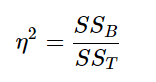
Eta-square is reported as percentage of variance of the outcome/dependent variable explained by the predictor/independent variable.
Although you report variance explained by the predictor/independent variable, you can also use the 𝜂2 guidelines for effect size:
| 𝜂2 | Size |
| 0.01 | Small |
| 0.09 | Medium |
| 0.25 | Large |
| Note: if less than .01, no effect is reported |
Example continued adding on effect size for scores on job application tests
For our example, SS B =8246 and SS T = 11266, our values give an effect size, 𝜂2, of:
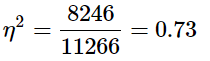
So, we are able to explain 73% of the variance in job test scores based on education. This is, in fact, a huge effect size, and most of the time we will not explain nearly that much variance.
So, we found that not only do we have a statistically significant result, but that our observed effect was very large! However, we still do not know specifically which groups are different from each other. It could be that they are all different, or that only those who have a relevant degree are different from the others, or that only those who have no degree are different from the others. To find out which is true, we need to do a special analysis called a post hoc test.
Post Hoc Tests
A post hoc test is used only after we find a statistically significant result and need to determine where our differences truly came from. The term “post hoc” comes from the Latin for “after the event”. There are many different post hoc tests that have been developed, and most of them will give us similar answers.
Bonferroni Test
A Bonferroni test is perhaps the simplest post hoc analysis. A Bonferroni test is a series of t -tests performed on each pair of groups. As we discussed earlier, the number of groups quickly grows the number of comparisons, which inflates Type I error rates. To avoid this, a Bonferroni test divides our significance level α by the number of comparisons we are making so that when they are all run, they sum back up to our original Type I error rate. Once we have our new significance level, we simply run independent samples t -tests to look for difference between our pairs of groups. This adjustment is sometimes called a Bonferroni Correction, and it is easy to do by hand if we want to compare obtained p -values to our new corrected α level, but it is more difficult to do when using critical values like we do for our analyses so we will leave our discussion of it to that.
Tukey’s Honest Significant Difference
Tukey’s Honest Significant Difference (HSD) is a very popular post hoc analysis. This analysis, like Bonferroni’s, makes adjustments based on the number of comparisons, but it makes adjustments to the test statistic when running the comparisons of two groups. These comparisons give us an estimate of the difference between the groups and a confidence interval for the estimate. We use this confidence interval in the same way that we use a confidence interval for a regular independent samples t -test: if it contains 0.00, the groups are not different, but if it does not contain 0.00 then the groups are different.
Example continued adding on post hoc for scores on job application tests: Tukey
Remember we are comparing scores from those whom applied for a single job opening: those with no college degree (none), those with a college degree that is not related to the job opening (unrelated), and those with a college degree from a relevant field (relevant).
Below are the differences between the group means and the Tukey’s HSD confidence intervals for the differences:
| Comparison | Difference | Tukey’s HSD CI |
| None vs Relevant | 40.60 | (28.87, 52.33) |
| None vs Unrelated | 19.50 | (7.77, 31.23) |
| Relevant vs Unrelated | 21.10 | (9.37, 32.83) |
As we can see, none of these intervals contain 0.00, so we can conclude that all three groups are different from one another.
Scheffe’s Test
Another common post hoc test is Scheffe’s Test. Like Tukey’s HSD, Scheffe’s test adjusts the test statistic for how many comparisons are made, but it does so in a slightly different way. The result is a test that is “conservative,” which means that it is less likely to commit a Type I Error, but this comes at the cost of less power to detect effects. We can see this by looking at the confidence intervals that Scheffe’s test gives us for our example.
Example continued adding on post hoc for scores on job application tests: Scheffe
Below are the differences between the group means and the Sheffe confidence intervals for the differences:
| Comparison | Difference | Scheffe’s CI |
| None vs Relevant | 40.60 | (28.35, 52.85) |
| None vs Unrelated | 19.50 | (7.25, 31.75) |
| Relevant vs Unrelated | 21.10 | (8.85, 33.35) |
As we can see, these are slightly wider than the intervals we got from Tukey’s HSD. This means that, all other things being equal, they are more likely to contain zero. In our case, however, the results are the same, and we again conclude that all three groups differ from one another.
There are many more post hoc tests than just these three, and they all approach the task in different ways, with some being more conservative and others being more powerful. In general, though, they will give highly similar answers. What is important here is to be able to interpret a post hoc analysis. If you are given post hoc analysis confidence intervals, like the ones seen above, read them the same way we read confidence intervals previously comparing two groups: if they contain zero, there is no difference; if they do not contain zero, there is a difference.
Other ANOVA Designs
We have only just scratched the surface on ANOVA in this chapter. There are many other variations available for the one-way ANOVA presented here. There are also other types of ANOVAs that you are likely to encounter. The first is called a factorial ANOVA . Factorial ANOVAs use multiple grouping variables, not just one, to look for group mean differences. Just as there is no limit to the number of groups in a one-way ANOVA, there is no limit to the number of grouping variables in a Factorial ANOVA, but it becomes very difficult to find and interpret significant results with many factors, so usually they are limited to two or three grouping variables with only a small number of groups in each. Another ANOVA is called a Repeated Measures ANOVA. This is an extension of a repeated measures or matched pairs t -test, but in this case we are measuring each person three or more times to look for a change. We can even combine both of these advanced ANOVAs into mixed designs to test very specific and valuable questions. These topics are far beyond the scope of this text, but you should know about their existence. Our treatment of ANOVA here is a small first step into a much larger world!
Learning Objectives
Having read the chapter, students should be able to:
- understand the basic purpose for analysis of variance (ANOVA) and the general logic that underlies the statistical procedure
- perform an ANOVA to evaluate data from a single factor, between subjects research design
- understand when post hoc tests are necessary and purpose that they serve
- calculate and interpret effect size
Exercises – Ch. 14
- What are the three pieces of variance analyzed in ANOVA?
- What does rejecting the null hypothesis in ANOVA tell us? What does it not tell us?
- What is the purpose of post hoc tests?
- Based on the ANOVA table below, do you reject or fail to reject the null hypothesis? What is the effect size?
| Source | SS | df | MS | F |
| Between | 60.72 | 3 | 20.24 | 3.88 |
| Within | 213.61 | 41 | 5.21 |
|
| Total | 274.33 | 44 |
|
|
5. Finish filling out the following ANOVA tables:
Problem 1: N = 14
| Source | SS | df | MS | F |
| Between |
| 2 | 14.10 |
|
| Within |
|
|
|
|
| Total | 64.65 |
|
|
|
| Source | SS | df | MS | F |
| Between |
| 2 |
| 42.36 |
| Within |
| 54 | 2.48 |
|
| Total |
|
|
|
|
6. You know that stores tend to charge different prices for similar or identical products, and you want to test whether or not these differences are, on average, statistically significantly different. You go online and collect data from 3 different stores, gathering information on 15 products at each store. You find that the average prices at each store are: Store 1 M = $27.82, Store 2 M= $38.96, and Store 3 M = $24.53. Based on the overall variability in the products and the variability within each store, you find the following values for the Sums of Squares: SST = 683.22, SSW = 441.19. Complete the ANOVA table and use the 4 step hypothesis testing procedure to see if there are systematic price differences between the stores.
7. You and your friend are debating which type of candy is the best. You find data on the average rating for hard candy (e.g. jolly ranchers, ̅X = 3.60), chewable candy (e.g. starburst, ̅X = 4.20), and chocolate (e.g. snickers, ̅X = 4.40); each type of candy was rated by 30 people. Test for differences in average candy rating using SSB = 16.18 and SSW = 28.74.
8. Administrators at a university want to know if students in different majors are more or less extroverted than others. They provide you with data they have for English majors (̅X = 3.78, n = 45), History majors (̅X = 2.23, n = 40), Psychology majors (̅X = 4.41, n = 51), and Math majors (̅X = 1.15, n = 28). You find the SSB = 75.80 and SSW = 47.40 and test at α = 0.05.
9. You are assigned to run a study comparing a new medication (̅X = 17.47, n = 19), an existing medication (̅X = 17.94, n = 18), and a placebo (̅X = 13.70, n= 20), with higher scores reflecting better outcomes. Use SSB = 210.10 and SSW = 133.90 to test for differences.
10. You are in charge of assessing different training methods for effectiveness. You have data on 4 methods: Method 1 (̅X = 87, n = 12), Method 2 (̅X = 92, n = 14), Method 3 (̅X = 88, n = 15), and Method 4 (̅X = 75, n = 11). Test for differences among these means, assuming SSB = 64.81 and SST = 399.45.
Answers to Odd- Numbered Exercises – Ch. 14
1. Variance between groups (SSB), variance within groups (SSW) and total variance (SST).
3. Post hoc tests are run if we reject the null hypothesis in ANOVA; they tell us which specific group differences are significant. 5. Finish filling out the following ANOVA tables:
| Source | SS | df | MS | F |
| Between | 28.20 | 2 | 14.10 | 4.26 |
| Within | 36.45 | 11 | 3.31 |
|
| Total | 64.65 | 13 |
|
|
| Source | SS | df | MS | F |
| Between | 210.10 | 2 | 105.05 | 42.36 |
| Within | 133.92 | 54 | 2.48 |
|
| Total | 344.02 |
|
|
|
7. Step 1: H 0 : μ 1 = μ 2 = μ 3 “There is no difference in average rating of candy quality”, H A : “At least one mean is different.”
Step 3: based on the given SSB and SSW and the computed df from step 2, is:
| Source | SS | df | MS | F |
| Between | 16.18 | 2 | 8.09 | 24.52 |
| Within | 28.74 | 87 | 0.33 |
|
| Total | 44.92 | 89 |
|
|
Step 4: F > F*, reject H 0 . Based on the data in our 3 groups, we can say that there is a statistically significant difference in the quality of different types of candy, F(2,87) = 24.52, p < .05. Since the result is significant, we need an effect size: η 2 = 16.18/44.92 = .36, which is a large effect.
| Source | SS | df | MS | F |
| Between | 210.10 | 2 | 105.02 | 42.36 |
| Within | 133.90 | 54 | 2.48 |
|
| Total | 344.00 | 56 |
|
|
Step 4: F > F*, reject H 0 . Based on the data in our 3 groups, we can say that there is a statistically significant difference in the effectiveness of the treatments, F(2,54) = 42.36, p < .05. Since the result is significant, we need an effect size: η 2 = 210.10/344.00 = .61, which is a large effect.
Introduction to Statistics for Psychology Copyright © 2021 by Alisa Beyer is licensed under a Creative Commons Attribution-NonCommercial-ShareAlike 4.0 International License , except where otherwise noted.
Share This Book
13.4 Test of Two Variances
Another use of the F distribution is testing two variances. It is often desirable to compare two variances rather than two averages. For instance, college administrators would like two college professors grading exams to have the same variation in their grading. For a lid to fit a container, the variation in the lid and the container should be the same. A supermarket might be interested in the variability of check-out times for two checkers.
To perform a F test of two variances, it is important that the following are true:
- The populations from which the two samples are drawn are normally distributed.
- The two populations are independent of each other.
Unlike most other tests in this book, the F test for equality of two variances is very sensitive to deviations from normality. If the two distributions are not normal, the test can give higher p -values than it should, or lower ones, in ways that are unpredictable. Many texts suggest that students not use this test at all, but in the interest of completeness we include it here.
Suppose we sample randomly from two independent normal populations. Let σ 1 2 σ 1 2 and σ 2 2 σ 2 2 be the population variances and s 1 2 s 1 2 and s 2 2 s 2 2 be the sample variances. Let the sample sizes be n 1 and n 2 . Since we are interested in comparing the two sample variances, we use the F ratio
F = [ ( s 1 ) 2 ( σ 1 ) 2 ] [ ( s 2 ) 2 ( σ 2 ) 2 ] . F = [ ( s 1 ) 2 ( σ 1 ) 2 ] [ ( s 2 ) 2 ( σ 2 ) 2 ] .
F has the distribution F ~ F ( n 1 – 1, n 2 – 1),
where n 1 – 1 are the degrees of freedom for the numerator and n 2 – 1 are the degrees of freedom for the denominator.
If the null hypothesis is σ 1 2 = σ 2 2 σ 1 2 = σ 2 2 , then the F ratio becomes F = [ ( s 1 ) 2 ( σ 1 ) 2 ] [ ( s 2 ) 2 ( σ 2 ) 2 ] = ( s 1 ) 2 ( s 2 ) 2 F = [ ( s 1 ) 2 ( σ 1 ) 2 ] [ ( s 2 ) 2 ( σ 2 ) 2 ] = ( s 1 ) 2 ( s 2 ) 2 .
The F ratio could also be ( s 2 ) 2 ( s 1 ) 2 ( s 2 ) 2 ( s 1 ) 2 . It depends on H a and on which sample variance is larger.
If the two populations have equal variances, then s 1 2 s 1 2 and s 2 2 s 2 2 are close in value and F = ( s 1 ) 2 ( s 2 ) 2 F = ( s 1 ) 2 ( s 2 ) 2 is close to 1. But if the two population variances are very different, s 1 2 s 1 2 and s 2 2 s 2 2 tend to be very different, too. Choosing s 1 2 s 1 2 as the larger sample variance causes the ratio ( s 1 ) 2 ( s 2 ) 2 ( s 1 ) 2 ( s 2 ) 2 to be greater than 1. If s 1 2 s 1 2 and s 2 2 s 2 2 are far apart, then F = ( s 1 ) 2 ( s 2 ) 2 F = ( s 1 ) 2 ( s 2 ) 2 is a large number.
Therefore, if F is close to 1, the evidence favors the null hypothesis (the two population variances are equal). But if F is much larger than 1, then the evidence is against the null hypothesis. A test of two variances may be left-tailed, right-tailed, or two-tailed.
Example 13.5
Two college instructors are interested in whethe there is any variation in the way they grade math exams. They each grade the same set of 30 exams. The first instructor’s grades have a variance of 52.3. The second instructor’s grades have a variance of 89.9. Test the claim that the first instructor’s variance is smaller. In most colleges, it is desirable for the variances of exam grades to be nearly the same among instructors. The level of significance is 10 percent.
Let 1 and 2 be the subscripts that indicate the first and second instructor, respectively.
n 1 = n 2 = 30.
H 0 : σ 1 2 = σ 2 2 σ 1 2 = σ 2 2 and H a : σ 1 2 < σ 2 2 σ 1 2 < σ 2 2 .
Calculate the test statistic: By the null hypothesis ( σ 1 2 = σ 2 2 ) ( σ 1 2 = σ 2 2 ) , the F statistic is
F = [ ( s 1 ) 2 ( σ 1 ) 2 ] [ ( s 2 ) 2 ( σ 2 ) 2 ] = ( s 1 ) 2 ( s 2 ) 2 = 52.3 89.9 = 0.5818. F = [ ( s 1 ) 2 ( σ 1 ) 2 ] [ ( s 2 ) 2 ( σ 2 ) 2 ] = ( s 1 ) 2 ( s 2 ) 2 = 52.3 89.9 = 0.5818.
Distribution for the test: F 29,29 where n 1 – 1 = 29 and n 2 – 1 = 29.
Graph: This test is left-tailed.
Draw the graph, labeling and shading appropriately.
Probability statement: p -value = P ( F < 0.5818) = 0.0753.
Compare α and the p -value: α = 0.10; α > p -value.
Make a decision: Since α > p -value, reject H 0 .
Conclusion: With a 10 percent level of significance from the data, there is sufficient evidence to conclude that the variance in grades for the first instructor is smaller.
Using the TI-83, 83+, 84, 84+ Calculator
Press STAT and arrow over to TESTS . Arrow down to D:2-SampFTest . Press ENTER . Arrow to Stats and press ENTER . For Sx1 , n1 , Sx2 , and n2 , enter ( 52.3 ) ( 52.3 ) , 30 , ( 89.9 ) ( 89.9 ) , and 30 . Press ENTER after each. Arrow to σ1: and < σ2 . Press ENTER . Arrow down to Calculate and press ENTER . F = 0.5818 and p -value = 0.0753. Do the procedure again and try Draw instead of Calculate .
Try It 13.5
The New York Choral Society divides male singers into four categories from highest voices to lowest: Tenor1, Tenor2, Bass1, and Bass2. In the table are heights of the men in the Tenor1 and Bass2 groups. One suspects that taller men will have lower voices, and that the variance of height may go up with the lower voices as well. Do we have good evidence that the variance of the heights of singers in each of these two groups (Tenor1 and Bass2) are different?
| Tenor1 | Bass2 | Tenor1 | Bass2 | Tenor1 | Bass2 |
|---|---|---|---|---|---|
| 69 | 72 | 67 | 72 | 68 | 67 |
| 72 | 75 | 70 | 74 | 67 | 70 |
| 71 | 67 | 65 | 70 | 64 | 70 |
| 66 | 75 | 72 | 66 | 69 | |
| 76 | 74 | 70 | 68 | 72 | |
| 74 | 72 | 68 | 75 | 71 | |
| 71 | 72 | 64 | 68 | 74 | |
| 66 | 74 | 73 | 70 | 75 | |
| 68 | 72 | 66 | 72 |
This book may not be used in the training of large language models or otherwise be ingested into large language models or generative AI offerings without OpenStax's permission.
Want to cite, share, or modify this book? This book uses the Creative Commons Attribution License and you must attribute Texas Education Agency (TEA). The original material is available at: https://www.texasgateway.org/book/tea-statistics . Changes were made to the original material, including updates to art, structure, and other content updates.
Access for free at https://openstax.org/books/statistics/pages/1-introduction
- Authors: Barbara Illowsky, Susan Dean
- Publisher/website: OpenStax
- Book title: Statistics
- Publication date: Mar 27, 2020
- Location: Houston, Texas
- Book URL: https://openstax.org/books/statistics/pages/1-introduction
- Section URL: https://openstax.org/books/statistics/pages/13-4-test-of-two-variances
© Apr 16, 2024 Texas Education Agency (TEA). The OpenStax name, OpenStax logo, OpenStax book covers, OpenStax CNX name, and OpenStax CNX logo are not subject to the Creative Commons license and may not be reproduced without the prior and express written consent of Rice University.
User Preferences
Content preview.
Arcu felis bibendum ut tristique et egestas quis:
- Ut enim ad minim veniam, quis nostrud exercitation ullamco laboris
- Duis aute irure dolor in reprehenderit in voluptate
- Excepteur sint occaecat cupidatat non proident
Keyboard Shortcuts
10.1 - z-test: when population variance is known.
Let's start by acknowledging that it is completely unrealistic to think that we'd find ourselves in the situation of knowing the population variance, but not the population mean. Therefore, the hypothesis testing method that we learn on this page has limited practical use. We study it only because we'll use it later to learn about the "power" of a hypothesis test (by learning how to calculate Type II error rates). As usual, let's start with an example.
Example 10-1 Section

Boys of a certain age are known to have a mean weight of \(\mu=85\) pounds. A complaint is made that the boys living in a municipal children's home are underfed. As one bit of evidence, \(n=25\) boys (of the same age) are weighed and found to have a mean weight of \(\bar{x}\) = 80.94 pounds. It is known that the population standard deviation \(\sigma\) is 11.6 pounds (the unrealistic part of this example!). Based on the available data, what should be concluded concerning the complaint?
The null hypothesis is \(H_0:\mu=85\), and the alternative hypothesis is \(H_A:\mu<85\). In general, we know that if the weights are normally distributed, then:
\(Z=\dfrac{\bar{X}-\mu}{\sigma/\sqrt{n}}\)
follows the standard normal \(N(0,1)\) distribution. It is actually a bit irrelevant here whether or not the weights are normally distributed, because the same size \(n=25\) is large enough for the Central Limit Theorem to apply. In that case, we know that \(Z\), as defined above, follows at least approximately the standard normal distribution. At any rate, it seems reasonable to use the test statistic:
\(Z=\dfrac{\bar{X}-\mu_0}{\sigma/\sqrt{n}}\)
for testing the null hypothesis
\(H_0:\mu=\mu_0\)
against any of the possible alternative hypotheses \(H_A:\mu \neq \mu_0\), \(H_A:\mu<\mu_0\), and \(H_A:\mu>\mu_0\).
For the example in hand, the value of the test statistic is:
\(Z=\dfrac{80.94-85}{11.6/\sqrt{25}}=-1.75\)
The critical region approach tells us to reject the null hypothesis at the \(\alpha=0.05\) level if \(Z<-1.645\). Therefore, we reject the null hypothesis because \(Z=-1.75<-1.645\), and therefore falls in the rejection region:
As always, we draw the same conclusion by using the \(p\)-value approach. Recall that the \(p\)-value approach tells us to reject the null hypothesis at the \(\alpha=0.05\) level if the \(p\)-value \(\le \alpha=0.05\). In this case, the \(p\)-value is \(P(Z<-1.75)=0.0401\):
As expected, we reject the null hypothesis because the \(p\)-value \(=0.0401<\alpha=0.05\).
By the way, we'll learn how to ask Minitab to conduct the \(Z\)-test for a mean \(\mu\) in a bit, but this is what the Minitab output for this example looks like this:
| N | Mean | SE Mean | 95% Upper Bound | Z | P |
|---|---|---|---|---|---|
| 25 | 80.9400 | 2.3200 | 84.7561 | -1.75 | 0.040 |
Have a language expert improve your writing
Run a free plagiarism check in 10 minutes, generate accurate citations for free.
- Knowledge Base
Variability | Calculating Range, IQR, Variance, Standard Deviation
Published on September 7, 2020 by Pritha Bhandari . Revised on June 21, 2023.
Variability describes how far apart data points lie from each other and from the center of a distribution. Along with measures of central tendency , measures of variability give you descriptive statistics that summarize your data.
Variability is also referred to as spread, scatter or dispersion. It is most commonly measured with the following:
- Range : the difference between the highest and lowest values
- Interquartile range : the range of the middle half of a distribution
- Standard deviation : average distance from the mean
- Variance : average of squared distances from the mean
Table of contents
Why does variability matter, interquartile range, standard deviation, what’s the best measure of variability, other interesting articles, frequently asked questions about variability.
While the central tendency , or average, tells you where most of your points lie, variability summarizes how far apart they are. This is important because the amount of variability determines how well you can generalize results from the sample to your population.
Low variability is ideal because it means that you can better predict information about the population based on sample data. High variability means that the values are less consistent, so it’s harder to make predictions.
Data sets can have the same central tendency but different levels of variability or vice versa . If you know only the central tendency or the variability, you can’t say anything about the other aspect. Both of them together give you a complete picture of your data.
Using simple random samples , you collect data from 3 groups:
- Sample A: high school students,
- Sample B: college students,
- Sample C: adult full-time employees.

All three of your samples have the same average phone use, at 195 minutes or 3 hours and 15 minutes. This is the x-axis value where the peak of the curves are.
Here's why students love Scribbr's proofreading services
Discover proofreading & editing
The range tells you the spread of your data from the lowest to the highest value in the distribution. It’s the easiest measure of variability to calculate.
To find the range , simply subtract the lowest value from the highest value in the data set.
| Data (minutes) | 72 | 110 | 134 | 190 | 238 | 287 | 305 | 324 |
|---|
The highest value ( H ) is 324 and the lowest ( L ) is 72 .
R = 324 – 72 = 252
The range of your data is 252 minutes .
Because only 2 numbers are used, the range is influenced by outliers and doesn’t give you any information about the distribution of values. It’s best used in combination with other measures.
The interquartile range gives you the spread of the middle of your distribution.
For any distribution that’s ordered from low to high, the interquartile range contains half of the values. While the first quartile (Q1) contains the first 25% of values, the fourth quartile (Q4) contains the last 25% of values.

The interquartile range is the third quartile (Q3) minus the first quartile (Q1). This gives us the range of the middle half of a data set.
Multiply the number of values in the data set (8) by 0.25 for the 25th percentile (Q1) and by 0.75 for the 75th percentile (Q3).
Q1 position: 0.25 x 8 = 2
Q3 position: 0.75 x 8 = 6
Q1 is the value in the 2nd position, which is 110 . Q3 is the value in the 6th position, which is 287 .
IQR = Q3 – Q1
IQR = 287 – 110 = 177
The interquartile range of your data is 177 minutes .
Just like the range, the interquartile range uses only 2 values in its calculation. But the IQR is less affected by outliers : the 2 values come from the middle half of the data set, so they are unlikely to be extreme scores.
The IQR gives a consistent measure of variability for skewed as well as normal distributions.
Five-number summary
Every distribution can be organized using a five-number summary :
- Lowest value
- Q1: 25th percentile
- Q2: the median
- Q3: 75th percentile
- Highest value (Q4)
These five-number summaries can be easily visualized using box and whisker plots.

The standard deviation is the average amount of variability in your dataset.
It tells you, on average, how far each score lies from the mean. The larger the standard deviation, the more variable the data set is.
There are six steps for finding the standard deviation by hand:
- List each score and find their mean .
- Subtract the mean from each score to get the deviation from the mean.
- Square each of these deviations.
- Add up all of the squared deviations.
- Divide the sum of the squared deviations by n – 1 (for a sample ) or N (for a population).
- Find the square root of the number you found.
| Step 1: Data (minutes) | Step 2: Deviation from mean | Steps 3 + 4: Squared deviation |
|---|---|---|
| 72 | 72 – 207.5 = -135.5 | 18360.25 |
| 110 | 110 – 207.5 = -97.5 | 9506.25 |
| 134 | 134 – 207.5 = -73.5 | 5402.25 |
| 190 | 190 – 207.5 = -17.5 | 306.25 |
| 238 | 238 – 207.5 = 30.5 | 930.25 |
| 287 | 287 – 207.5 = 79.5 | 6320.25 |
| 305 | 305 – 207.5 = 97.5 | 9506.25 |
| 324 | 324 – 207.5 = 116.5 | 13572.25 |
| Mean = | Sum = 0 | Sum of squares = |
63904 / 7 = 9129.14
s = √9129.14 = 95.54
The standard deviation of your data is 95.54 . This means that on average, each score deviates from the mean by 95.54 points.
Standard deviation formula for populations
If you have data from the entire population, use the population standard deviation formula:
| Formula | Explanation |
|---|---|
| = population standard deviation = sum of… = each value = population mean = number of values in the population |
Standard deviation formula for samples
If you have data from a sample, use the sample standard deviation formula:
| Formula | Explanation |
|---|---|
| = sample standard deviation = sum of… = each value = sample mean = number of values in the sample |
Why use n – 1 for sample standard deviation?
Samples are used to make statistical inferences about the population that they came from.
When you have population data, you can get an exact value for population standard deviation. Since you collect data from every population member, the standard deviation reflects the precise amount of variability in your distribution, the population.
But when you use sample data, your sample standard deviation is always used as an estimate of the population standard deviation. Using n in this formula tends to give you a biased estimate that consistently underestimates variability.
Reducing the sample n to n – 1 makes the standard deviation artificially large, giving you a conservative estimate of variability.
While this is not an unbiased estimate, it is a less biased estimate of standard deviation: it is better to overestimate rather than underestimate variability in samples.
The difference between biased and conservative estimates of standard deviation gets much smaller when you have a large sample size.
The variance is the average of squared deviations from the mean. A deviation from the mean is how far a score lies from the mean.
Variance is the square of the standard deviation. This means that the units of variance are much larger than those of a typical value of a data set.
While it’s harder to interpret the variance number intuitively, it’s important to calculate variance for comparing different data sets in statistical tests like ANOVAs .
Variance reflects the degree of spread in the data set. The more spread the data, the larger the variance is in relation to the mean.
s 2 = 95.5 x 95.5 = 9129.14
The variance of your data is 9129.14 .
To find the variance by hand, perform all of the steps for standard deviation except for the final step.
Variance formula for populations
| Formula | Explanation |
|---|---|
| = population variance = sum of… = each value = population mean = number of values in the population |
Variance formula for samples
| Formula | Explanation |
|---|---|
| = sample variance = sum of… = each value = sample mean = number of values in the sample |
Biased versus unbiased estimates of variance
An unbiased estimate in statistics is one that doesn’t consistently give you either high values or low values – it has no systematic bias.
Just like for standard deviation, there are different formulas for population and sample variance. But while there is no unbiased estimate for standard deviation, there is one for sample variance.
If the sample variance formula used the sample n , the sample variance would be biased towards lower numbers than expected. Reducing the sample n to n – 1 makes the variance artificially larger.
In this case, bias is not only lowered but totally removed. The sample variance formula gives completely unbiased estimates of variance.
So why isn’t the sample standard deviation also an unbiased estimate?
That’s because sample standard deviation comes from finding the square root of sample variance. Since a square root isn’t a linear operation, like addition or subtraction, the unbiasedness of the sample variance formula isn’t carried over the sample standard deviation formula.
The best measure of variability depends on your level of measurement and distribution.
Level of measurement
For data measured at an ordinal level, the range and interquartile range are the only appropriate measures of variability.
For more complex interval and ratio levels, the standard deviation and variance are also applicable.
Distribution
For normal distributions, all measures can be used. The standard deviation and variance are preferred because they take your whole data set into account, but this also means that they are easily influenced by outliers.
For skewed distributions or data sets with outliers, the interquartile range is the best measure. It’s least affected by extreme values because it focuses on the spread in the middle of the data set.
If you want to know more about statistics , methodology , or research bias , make sure to check out some of our other articles with explanations and examples.
- Student’s t table
- Student’s t distribution
- Quartiles & Quantiles
- Measures of central tendency
- Correlation coefficient
Methodology
- Cluster sampling
- Stratified sampling
- Types of interviews
- Cohort study
- Thematic analysis
Research bias
- Implicit bias
- Baader-Meinhof phenomenon
- Cognitive bias
- Survivorship bias
- Availability heuristic
- Nonresponse bias
- Regression to the mean
Variability tells you how far apart points lie from each other and from the center of a distribution or a data set.
Variability is also referred to as spread, scatter or dispersion.
Variability is most commonly measured with the following descriptive statistics :
While central tendency tells you where most of your data points lie, variability summarizes how far apart your points from each other.
Data sets can have the same central tendency but different levels of variability or vice versa . Together, they give you a complete picture of your data.
Descriptive statistics summarize the characteristics of a data set. Inferential statistics allow you to test a hypothesis or assess whether your data is generalizable to the broader population.
Cite this Scribbr article
If you want to cite this source, you can copy and paste the citation or click the “Cite this Scribbr article” button to automatically add the citation to our free Citation Generator.
Bhandari, P. (2023, June 21). Variability | Calculating Range, IQR, Variance, Standard Deviation. Scribbr. Retrieved September 16, 2024, from https://www.scribbr.com/statistics/variability/
Is this article helpful?

Pritha Bhandari
Other students also liked, how to find the range of a data set | calculator & formula, how to calculate standard deviation (guide) | calculator & examples, normal distribution | examples, formulas, & uses, what is your plagiarism score.
IMAGES
VIDEO
COMMENTS
The variability hypothesis, also known as the greater male variability hypothesis, ... For example, he highlights findings from the Novara Expedition of 1861-1867 where "a vast number of measurements of various parts of the body in different races were made, and the men were found in almost every case to present a greater range of variation ...
The specific test considered here is called analysis of variance (ANOVA) and is a test of hypothesis that is appropriate to compare means of a continuous variable in two or more independent comparison groups. For example, in some clinical trials there are more than two comparison groups.
One-Way ANOVA: The Process. A one-way ANOVA uses the following null and alternative hypotheses: H0 (null hypothesis): μ1 = μ2 = μ3 = … = μk (all the population means are equal) H1 (alternative hypothesis): at least one population mean is different from the rest. You will typically use some statistical software (such as R, Excel, Stata ...
ANOVA, which stands for Analysis of Variance, is a statistical test used to analyze the difference between the means of more than two groups. A one-way ANOVA uses one independent variable, while a two-way ANOVA uses two independent variables. As a crop researcher, you want to test the effect of three different fertilizer mixtures on crop yield.
There are two main types: one-way and two-way. Two-way tests can be with or without replication. One-way ANOVA between groups: used when you want to test two groups to see if there's a difference between them. Two way ANOVA without replication: used when you have one group and you're double-testing that same group.
Hypothesis Test about a Variance. When people think of statistical inference, they usually think of inferences involving population means or proportions. ... Thus, product quality is often defined in terms of low variability. Sample variance \(s^2\) can be used for inferences concerning a population variance \(\sigma^2\).
ANOVA is based on comparing the variance (or variation) between the data samples to the variation within each particular sample. If the between-group variance is high and the within-group variance is low, this provides evidence that the means of the groups are significantly different. ... Null Hypothesis (H0): This is the hypothesis that there ...
ANOVA (Analysis of Variance) is a statistical test used to analyze the difference between the means of more than two groups. A two-way ANOVA is used to estimate how the mean of a quantitative variable changes according to the levels of two categorical variables. Use a two-way ANOVA when you want to know how two independent variables, in ...
This page explains how to perform hypothesis tests about the variance of a normal distribution, called Chi-square tests. We analyze two different situations: when it is unknown. Depending on the situation, the Chi-square statistic used in the test has a different distribution. At the end of the page, we propose some solved exercises.
Lesson 12: Tests for Variances. Continuing our development of hypothesis tests for various population parameters, in this lesson, we'll focus on hypothesis tests for population variances. Specifically, we'll develop: a hypothesis test for testing whether a single population variance σ 2 equals a particular value.
The sum of squares, degrees of freedom and mean squares are organized in a table called an ANOVA table. Figure 11-1 below is a template for an ANOVA table. Figure 11-1: ANOVA table tamplate. Where: ˉχi = sample mean from the ith group. s2 i = sample variance from the ith group. ni = sample size from the ith group.
Present the findings in your results and discussion section. Though the specific details might vary, the procedure you will use when testing a hypothesis will always follow some version of these steps. Table of contents. Step 1: State your null and alternate hypothesis. Step 2: Collect data. Step 3: Perform a statistical test.
The test statistic is: χ2 = (n − 1)s2 σ2 (8.5.1) (8.5.1) χ 2 = (n − 1) s 2 σ 2. where: n n is the the total number of data. s2 s 2 is the sample variance. σ2 σ 2 is the population variance. You may think of s s as the random variable in this test. The number of degrees of freedom is df = n − 1 d f = n − 1. A test of a single ...
where: n = the total number of data ; s 2 = sample variance ; σ 2 = population variance; You may think of s as the random variable in this test. The number of degrees of freedom is df = n - 1.A test of a single variance may be right-tailed, left-tailed, or two-tailed. Example 11.10 will show you how to set up the null and alternative hypotheses. The null and alternative hypotheses contain ...
Additional Hypothesis Tests. In unit 1, we learned the basics of statistics - what they are, how they work, and the mathematical and conceptual principles that guide them. ... It is a ratio of two estimates of the population variance based on the sample data. Experiments are designed to determine if there is a cause and effect relationship ...
Introduction; 9.1 Null and Alternative Hypotheses; 9.2 Outcomes and the Type I and Type II Errors; 9.3 Distribution Needed for Hypothesis Testing; 9.4 Rare Events, the Sample, and the Decision and Conclusion; 9.5 Additional Information and Full Hypothesis Test Examples; 9.6 Hypothesis Testing of a Single Mean and Single Proportion; Key Terms; Chapter Review; Formula Review
The theoretical work for developing a hypothesis test for a population variance \(\sigma^2\) is already behind us. Recall that if you have a random sample of size n from a normal population with (unknown) mean \(\mu\) and variance \(\sigma^2\), ... and follow the standard hypothesis testing procedures. Let's take a look at an example.
Homogeneity of variance: the variance within each group being compared is similar among all groups. If one group has much more variation than others, it will limit the test's effectiveness. ... A Step-by-Step Guide with Easy Examples Hypothesis testing is a formal procedure for investigating our ideas about the world. It allows you to ...
The null hypothesis, denoted as H 0, is the hypothesis that the sample data occurs purely from chance. The alternative hypothesis, denoted as H 1 or H a, is the hypothesis that the sample data is influenced by some non-random cause. Hypothesis Tests. A hypothesis test consists of five steps: 1. State the hypotheses. State the null and ...
For the example in hand, the value of the test statistic is: Z = 80.94 − 85 11.6 / 25 = − 1.75. The critical region approach tells us to reject the null hypothesis at the α = 0.05 level if Z <− 1.645. Therefore, we reject the null hypothesis because Z = − 1.75 <− 1.645, and therefore falls in the rejection region: Z -1.645 -1.75.
Researchers commonly use analysis of variance (ANOVA) to statistically test results of factorial designs. Performing an a priori power analysis is crucial to ensure that the ANOVA is sufficiently powered, however, it often poses a challenge and can result in large sample sizes, especially if the expected effect size is small. Due to the high prevalence of small effect sizes in psychology ...
The variability concerns how spread out the values are. In descriptive statistics, there is no uncertainty - the statistics precisely describe the data that you collected. ... A Step-by-Step Guide with Easy Examples Hypothesis testing is a formal procedure for investigating our ideas about the world. It allows you to statistically test your ...
The test statistic is: χ2 = (n − 1)s2 σ2 (11.7.1) (11.7.1) χ 2 = (n − 1) s 2 σ 2. where: n n is the the total number of data. s2 s 2 is the sample variance. σ2 σ 2 is the population variance. You may think of s s as the random variable in this test. The number of degrees of freedom is df = n − 1 d f = n − 1.
Variance example To get variance, square the standard deviation. s = 95.5. s 2 = 95.5 x 95.5 = 9129.14. The variance of your data is 9129.14. ... Inferential statistics allow you to test a hypothesis or assess whether your data is generalizable to the broader population. Cite this Scribbr article.